open Table of Content
Table Of Contents
Introduction
Note: this is an in-progress post, I still have to refine some section and write some of them all (looking at you, clustering). The reason i’m posting it unfinished is because i don’t want it to stay laying untracked in my pc and maybe forgotten :)
ML definition (from Tom M.Mitchell in “Machine Learning” book from 1997):
A computer program A is said to learn from experience D with respect to some class of tasks T and perfomance measure L, if the performance of A at task in T, as measured by L, improves with experience D.
From this definition we can identify the 4 key elements of learning:
- The algorithm A. Aims to learn a solution of the task T using the experience D. It finds the solution in a set of possible solution $\mathcal{H}$ called hypothesis space. Learning aims to find the “best” $h \in \mathcal{H}$ from D according to L.
- The experience D. D is the dataset $D =\set{s_1,…,S_N}$ where $s_i \sim \tilde{P}$.
- The task T. This defines the structure of each sample $s_i$. For supervised task: $s_i=(x_i,y_i)$, for unsupervised task $s_i = x_i$.
- The performance measure L. $L(h,s)$ evaluates the goodness of $h$ on $s$.
Ideally, we want to find: $$\tilde{h} = \mathop{\arg \min}\limits_{h \in \mathcal{H}} \Big( TrueErr(h) = \int L(h,s)d\tilde{P}(s)\Big)$$ But this is computationally impossible due to the fact that the distribution $\tilde{P}$ is unknown. So instead we focus on an approximation:
$$h^* = \mathop{\arg \min}\limits_{h \in \mathcal{H}} \Big( TrainingErr(h) = \sum_{s\in D} L(h,s)\Big)$$
Inductive Leap
The ability of a model to perform well on unobserved samples is called generalisation. We can measure generalisation in this way:
- Split dataset in training and test $D = D_{tr} \cup D_{tst}$
- Minimize Training error over $D_{tr}$
- Calculate generalisation error over unseen samples $TestErr(h) = \sum_{s \in D_{tst}} L(h,s)$
Linear Regression
Let’s define:
- The dataset: $$D = \set{(x_i,y_i)}_{i=1,…,N}$$
- The loss measure: $$L(h,s=(x_i,y_i))= MSE(h,(x_i,y_i)) = (y_i - h(x_i))^2$$
- The hypothesis space:$$\mathcal{H}= \set{h|h:\mathbb{R}\rightarrow \mathbb{R} \text{ is linear}} = \set{h|wx: w \in \mathbb{R}}$$ We want to find best fitting line:
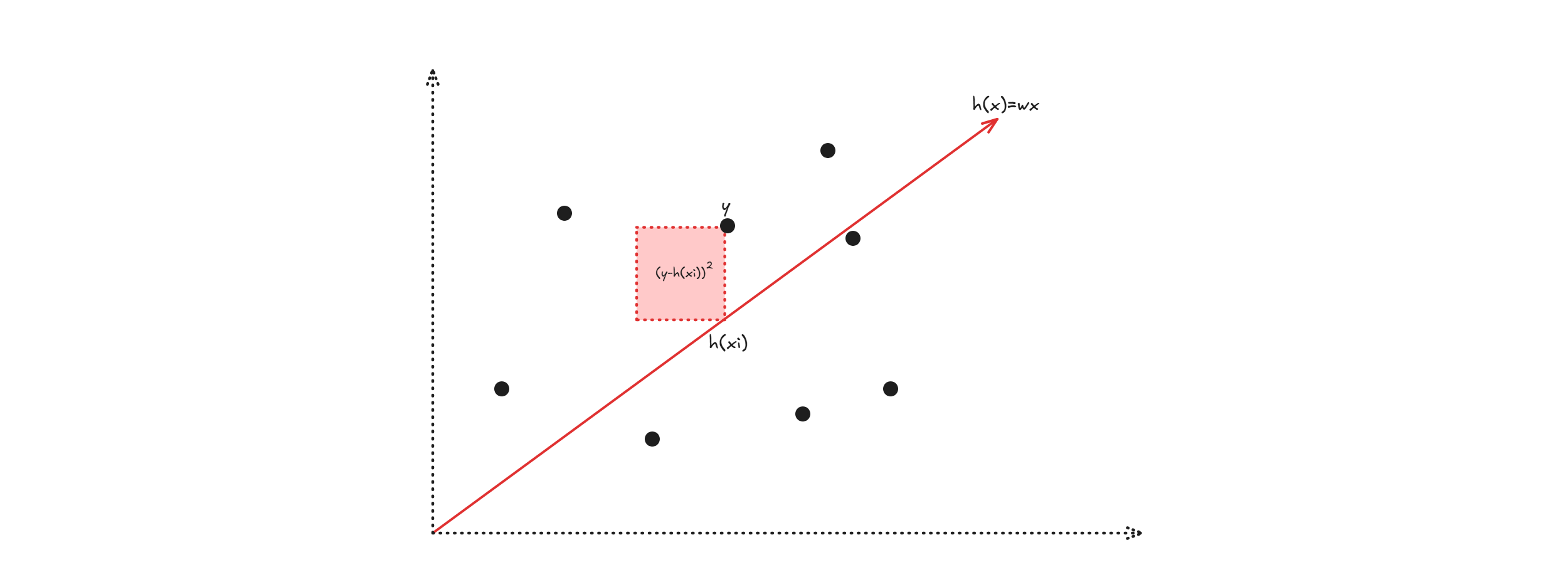
So we do:
$$h = \mathop{\arg \min}\limits_{h \in \mathcal{H}} \Big(TrainingErr(h) \Big)= \mathop{\arg \min}\limits_{h \in \mathcal{H}} \sum_{s \in D} L(h,s)$$$$ = \mathop{\arg \min}\limits_{h \in \mathcal{H}} MSE(h,s) = \mathop{\arg \min}\limits_{h \in \mathcal{H}} \sum_{i=1}^N (y_i-h(x_i))^2$$ Since you can write $h(x_i)$ as $wx_i$, then you can write
$$MSE(h,s) = \sum_{i=1}^N (y_i-h(x_i))^2 \equiv MSE(w,s)=\sum_{i=1}^N (y_i-wx_i)^2$$
To minimize
$$h = \mathop{\arg \min}\limits_{h \in \mathcal{H}} \Big(MSE(h,s)\Big) = \mathop{\arg \min}\limits_{w \in \mathbb{R}} \Big(MSE(w,s) = \frac{1}{N} \sum_{i=1}^N (y_i-wx_i)^2\Big)$$
You do
$$\nabla_w MSE(w,s) = 0$$ Since the function is convex there is a single minimum point: $$\nabla_w \frac{1}{N} \sum_{i=1}^N (y_i-wx_i)^2 = 0 = \frac{\partial \frac{1}{N} \sum_{i=1}^N (y_i-wx_i)^2}{\partial w} = \frac{1}{N} \sum_{i=1}^N 2(y_i - wx_i)(-x_i) = 0$$ $$\implies w = \frac{\sum_{i=1}^{N} x_iy_i}{\sum_{i=1}^N}x_i$$ If $x \in \mathbb{R}^n$, you can do the same calculation and obtain: $$w = (X^TX)^{-1}X^TY$$
Quadratic regression and beyond
For quadratic regression, the hypothesis space changes: $$\mathcal{H_2} = \set{h|h:\mathbb{R} \rightarrow \mathbb{R} \text{ is quadratic}} =\set{h| w_1x^2 +w_2x + w_3: w_1,w_2,w_3 \in \mathbb{R}}$$ But if you write the hypothesis space this way, you need to minimize 3 variables. To avoid that, you can use this trick:
- write $\phi(x) = (x^2, x, 1)^T$
- Then you can write $\mathcal{H_w} = {w^T \phi(x), w \in \mathbb{R}^3}$
The close form solution is: $w = (\Phi^T\Phi)^{-1}\Phi^TY$, where $\Phi = [\phi(x_1),…,\phi(x_n)]^T$
Probabilistic view on Linear regression
Linear regressin has a strict relation with Maximum likelihoot estimator: $$\theta_{MLE} = \mathop{\arg \max}\limits_{\theta \in \mathcal{P}} P(D|\theta)$$
where $P(D|\theta)$ is the data likelihood.
In linear regression we assume $$y = f(x) + \epsilon$$ where $\epsilon \sim \mathcal{N}(0,\sigma^2)$. We can assume error normality because the central limit theorem.
So if you suppose that $f(x) = w^Tx$, then you have that $y=w^Tx + \epsilon$ and that
$$y \sim \mathcal{N}(w^Tx,\sigma^2)$$
It can be proved that the maximizing data likelihood (MLE) is the same as minimizing loss in linear regression:
In fact (calculations done with $\sigma=1$): $$\theta_{MLE} = \mathop{\arg \max}\limits_{\theta \in \mathcal{P}} P(D|\theta) = \prod_{i=1}^N P(y|\theta) = \prod_{i=1}^{N} \frac{1}{\sqrt{2\pi}}exp\set{-\frac{(y_i-w^Tx_i)^2}{2}}$$ $$= \mathop{\arg \max}\limits_{w \in \mathbb{R}} -\sum_{i=1}^N log(\sqrt{2\pi}) - \sum_{i=1}^Nlog(\frac{(y_i-w^Tx_i)^2}{2}) = \mathop{\arg \max}\limits_{w \in \mathbb{R}} - \sum_{i=1}^N (y_i-w^Tx_i)^2$$
Which is the same as minimizing $\sum_{i=1}^N (y_i-w^Tx_i)^2$ as in linear regression.
Bias Variance Decomposition
In linear regression: $$h_0 \in \mathcal{H}_0 \implies h_0 \in \mathcal{H}_1 \implies h_0 \in \mathcal{H}_2$$ $$\implies \mathcal{H}_0 \subset \mathcal{H}_1 \subset \mathcal{H}_2$$ $$\implies TrainE(h_0) \geq TrainE(h_1) \geq TrainE(h_2)$$
This tells us that we can arbitrarly reduce training error by increasing model complexity.
But there is a trade off, in fact:
$$ExpectedTrueErr(h) = E_{\tilde{P}(D)}[TrueErr(h)]$$ $$ = B(h)^2 + V(h) + V(\epsilon)$$ This is called bias-variance decomposition.
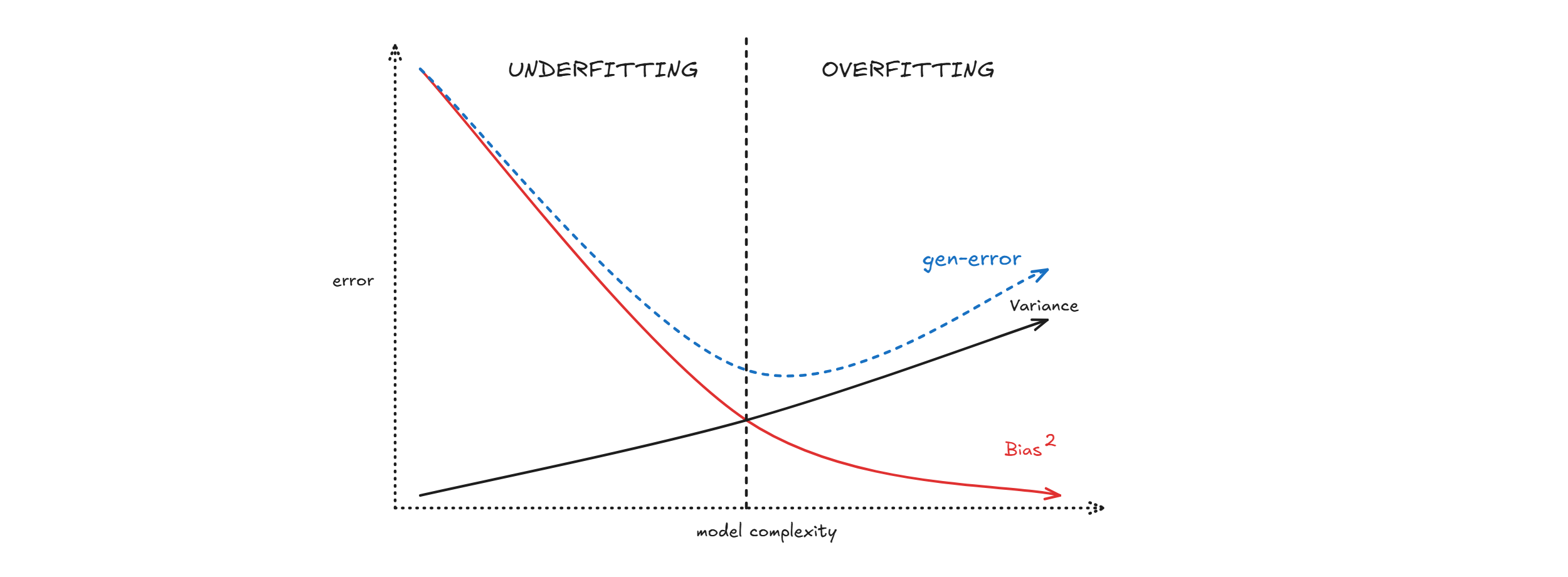
Measuring model complexity:
One way to measure the complexity of this model is with $0$-norm. $$|w|_0 = \text{ # } \set{x_i \neq 0} \text{ , for } i=1,…,M-1$$ So instead of minimizing only the loss, you can also minimize the model complexity:
$$w = \mathop{\arg \min}\limits_{w \in \mathbb{R}} \Big(TrainErr(w) + \overbrace{\lambda |w|_0}^{\text{penalisation term}}\Big)$$
For example if you consider $\mathcal{H_3}$ you have $h_3(x) = w_1x^3 + w_2x^2 + w_3x + w_4 = h_3$ and if you impose $|w|=0$ (only one entry must be not zero) then you can have:
$$h_3 = w_1x^3 + w_2x^2 + w_3x + w_4$$ $$h_2 = w_1 * 0 + w_2x^2 + w_3x + w_4$$ $$h_1 = w_1 * 0 + w_2 * 0 + w_3x + w_4$$ $$h_0 = w_1 * 0 + w_2 * 0 + w_3 * 0 + w_4$$
The problem with $0$-norm is that is not differentiable, so we use different norms:
Ridge regression
By taking $2$-norm (which is differentiable), you obtain ridge regression: $$w = \mathop{\arg \min}\limits_{w \in \mathbb{R}} (TrainE(w) + \lambda |w|_2)$$ Which has a closed form: $w = (X^TX+\lambda I)^{-1}X^Ty$
Lasso regression
By taging $1$-norm, you obtain lasso regression: $$w = \mathop{\arg \min}\limits_{w \in \mathbb{R}} (TrainE(w) + \lambda |w|_1)$$
probabilistic view on penalised model
As logistic regression has a strict tie with MLE, penalised model have a strict tie with MAP (Maximum Apriori estimator) $$\theta_{MAP} = \mathop{\arg \max}\limits_{\theta \in \mathcal{H}} P(\theta|D) = \mathop{\arg \max}\limits_{\theta \in D} P(D|\theta)P(\theta)$$ Where:
- $P(\theta|D)$ is the posterior.
- $P(D|\theta)$ is the data likelihood.
- $P(\theta)$ is the prior. It can be proved (in the same way as MLE) that maximizing $P(D|\theta)P(\theta)$ is equivalent to minimizing the $TrainErr(w) + \lambda|w|_k$ . With $P(w) = \mathcal{N}(0,\frac{1}{\lambda}I)$ we obtain ridge regression.
With $P(w) = \mathcal{L}(0,\frac{1}{\lambda}I)$ we obtain lasso regression.
Logistic regression
It is possible to think to use linear regression for a classification task in this way:
- use one-hot encoding for $y_i$, $y_i \in \mathbb{R} \implies one-hot(y_i) \in \mathbb{R}^c$
- find $w = (X^TX)^{-1}X^Ty$
- For prediction, you do $c = argmax_c h(x)[c]$ where $h(x) = x^t W$
So:
$$y = \begin{bmatrix} P(C=1|x) \cr P(C=2|x) \cr \vdots \cr P(C=K|x) \end{bmatrix} \approx \begin{bmatrix} w_1^Tx \cr w_2^Tx \cr \vdots \cr w_K^Tx \end{bmatrix}$$ But there is a problem, if we apporximate the probability of every class with a linear function we can happen to be in a situation like this:
True logistic regression
We fix the logarithm of a probability fraction given a fixed class to be linear
- $log(\frac{P(C=1|x)}{P(C=K|x)} \approx w_1^Tx$,
- $log(\frac{P(C=2|x)}{P(C=K|x)} \approx w_2^Tx$,
- …,
- $log(\frac{P(C=K|x)}{P(C=K|x)} = 0$
This way:
$$y = \begin{bmatrix} P(C=1|x) \cr P(C=2|x) \cr \vdots \cr P(C=K|x) \end{bmatrix} \approx \begin{bmatrix} e^{w_1^Tx} \cr e^{w_2^Tx} \cr \vdots \cr 1 \end{bmatrix}$$
The vector $y$ is not yet a probability distribution, so we have normalize it, we find that
$$P(C=c_i|x) = \frac{e^{w_i^Tx}}{1+ \sum_{i=1}^{K-1}e^{w_k^Tx}}$$
Training Logistic Regression
Taking the negative log likelihood as a loss function $(L = NLL)$.
$$L(w) = \sum_{i=1}^{N} - log(P(C=c_i|x_i) =-\sum_{i=1}^{N} log \Big(\frac{e^{w_{c_i}^Tx}}{1+ \sum_{i=1}^{K-1}e^{w_k^Tx}}\Big) = - \sum_{i=1}^N \Big[ w_{c_i}^T x_i - log(1+\sum_{k=1}^{K-1} e^{w_k^Tx_i}) \Big]$$
We can calculate $$\nabla_w L(w) = 0$$
$$\frac{\partial L(w)}{w_j} = - \sum_{i=1}^N \Big[ \frac{\partial(w_{c_i}^Tx_i)}{\partial w_j} - \frac{\partial}{\partial w_j} log(1+ \sum_{k=1}^{K-1} e^{{w_k}^Tx_i}) \Big]$$
$$= -\sum_{i=1}^{N} \left[ 1_{j=c_i} x_i - \frac{e^{w_j^T x_i}}{1 + \sum_{k=1}^{K-1} e^{w_k^T x_i}} x_i \right]$$
where $1_{j=c_i}$ is $1$ if $j=c_i$, 0 otherwise.
In compact form $$\frac{\partial L(w)}{\partial w_j} = \sum_{i=1}^{N} \left[ P(C=j|x_i) - 1_{j=c_i} \right] x_i$$
Since there is no closed form so we have to do gradient descent:
- $w_0 \in \mathbb{R}^n$
- for $t=1,…$
- $w_t = w_{t-1} - \alpha \nabla_{w_{t-1}} L(w)$
Perceptron
The idea is to find a separating hyperplane
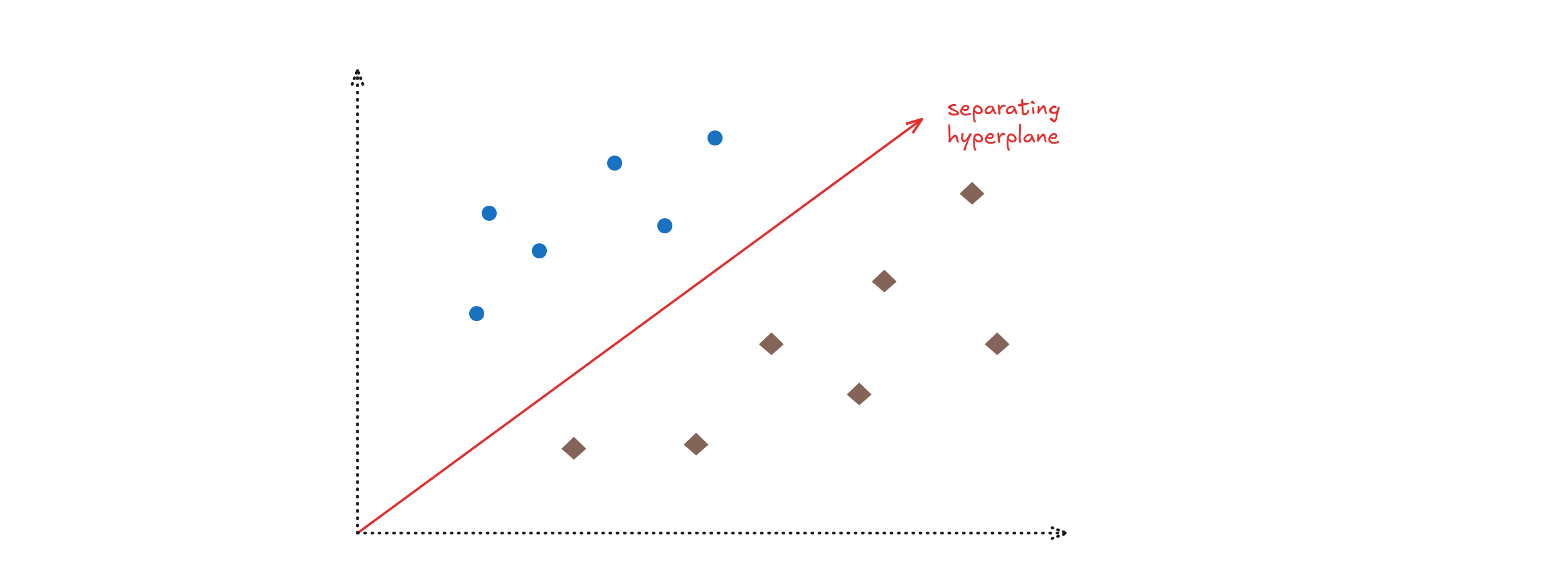
$x \in \mathbb{R}^n, w^Tx + b = 0$ is an hyperplane in $\mathbb{R}^n$ we take
$$h(x) = sign(w^Tx + b)$$
How to train perceptron
If $y$ is the real label then we have $4$ cases:
| $y$ | $w^Tx + b$ | $y(w^Tx + b)$ |
|---|---|---|
| >0 | >0 | >0 (no error) |
| >0 | <0 | <0 (error) |
| <0 | >0 | <0 (error) |
| <0 | <0 | >0 (no error) |
$$E_i(w,b) = -y_i(w^Tx_i + b)$$
$\nabla_w E_i = -y_ix_i$
$\nabla_b E_i = -y_i$
So we do:
- $w_t = w_{t-1} + \alpha y_ix_i$
- $b_t = b_{t-1} + \alpha y_i$
The algorithm is
- $w_0 \in \mathbb{R}^n$
- until convergence
- $\forall (x_i,y_i) \in D_{tr}$
- $y_i^* = sign(w^Tx_i + b)$
- if $y_i^* \neq y_i$
- $w_t = w_{t-1} + \alpha y_ix_i$
- $b_t = b_{t-1} + \alpha y_i$
Note: This is not gradient descent!
Support Vector Machine (SVM)
The idea behind SVM is finding the best separating hyperplane, i.e the one with highest margin.
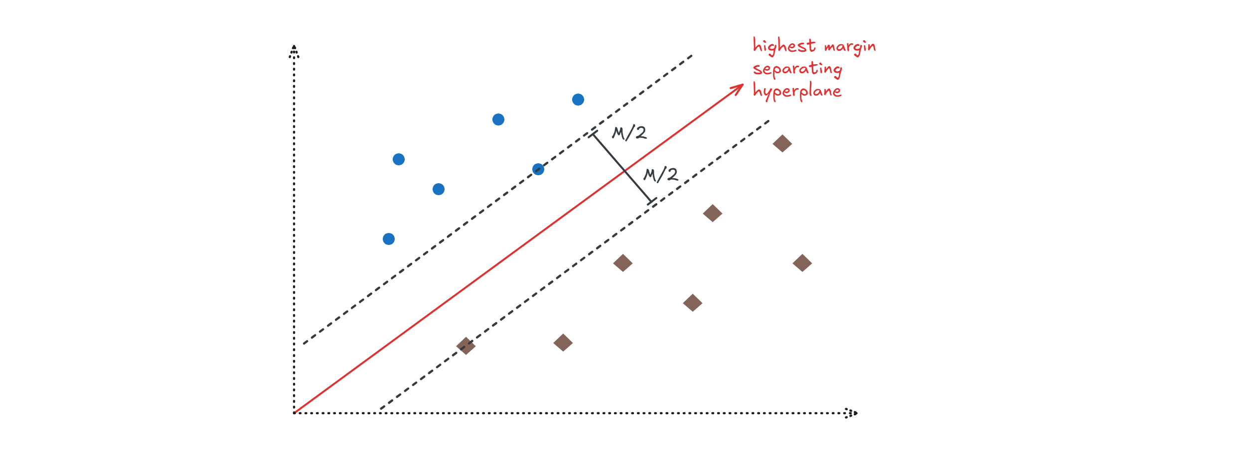
Preliminary:
- $L = \set{x |w^Tx + b = 0}$ is the set of point on a hyperplane
- We can prove that $dist_L(x) = \frac{1}{||w||}(w^Tx + b)$
If $y_i \in \set{-1,+1}$, i want:
- $dist_L(x) \geq M/2$ for $y_i = +1$
- $dist_L(x) \leq - M/2$ for $y_i = -1$ I can summarize this by saying $$y_i dist_L(x) \geq M/2$$ $$y_i \frac{1}{||w||}(w^Tx_i + b_i) \geq M/2$$ So we want to find:
$$\mathop{max}\limits_{w,b} M$$ $$\text{subject to } y_i \frac{1}{||w||}(w^Tx_i + b_i) \geq M/2, i = 1,…,N_{tr}$$ We can rewrite it as a minimization problem: $$y_i \frac{1}{||w||} (w^Tx_i + b_i) \geq M/2 \implies y_i (w^Tx_i + b_i) \geq \frac{M}{2} ||w|| \implies y_i (w^Tx_i + b_i) \geq 1 \text{ if } M = \frac{2}{||w||}$$ $$\mathop{max}\limits_{w,b} \Big(M = \frac{2}{||w||} \Big) = \mathop{min}\limits_{w,b} \Big(\frac{||w||}{2}\Big) = \mathop{min}\limits_{w,b} \Big(\frac{||w||_2^2}{2}\Big)$$
$$\text{subject to } y_i(w^Tx_i + b_i) - 1 \geq 0, i = 1,…,N_{tr}$$
You have then to solve the dual problem $$\mathop{max}\limits_{\lambda} \text{ }\mathop{inf}\limits_{w,b} \mathcal{L}(w,b,\lambda)$$
Beyond linear models, kernel trick
All linear models we have seen fails to learn the XOR operator
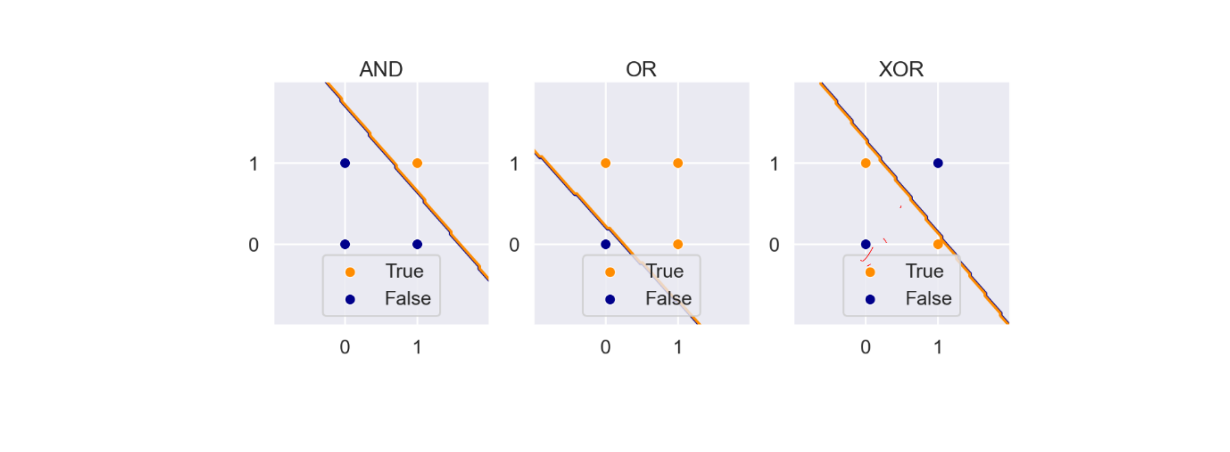
We would like to empower linear models to solve non-linear problems.
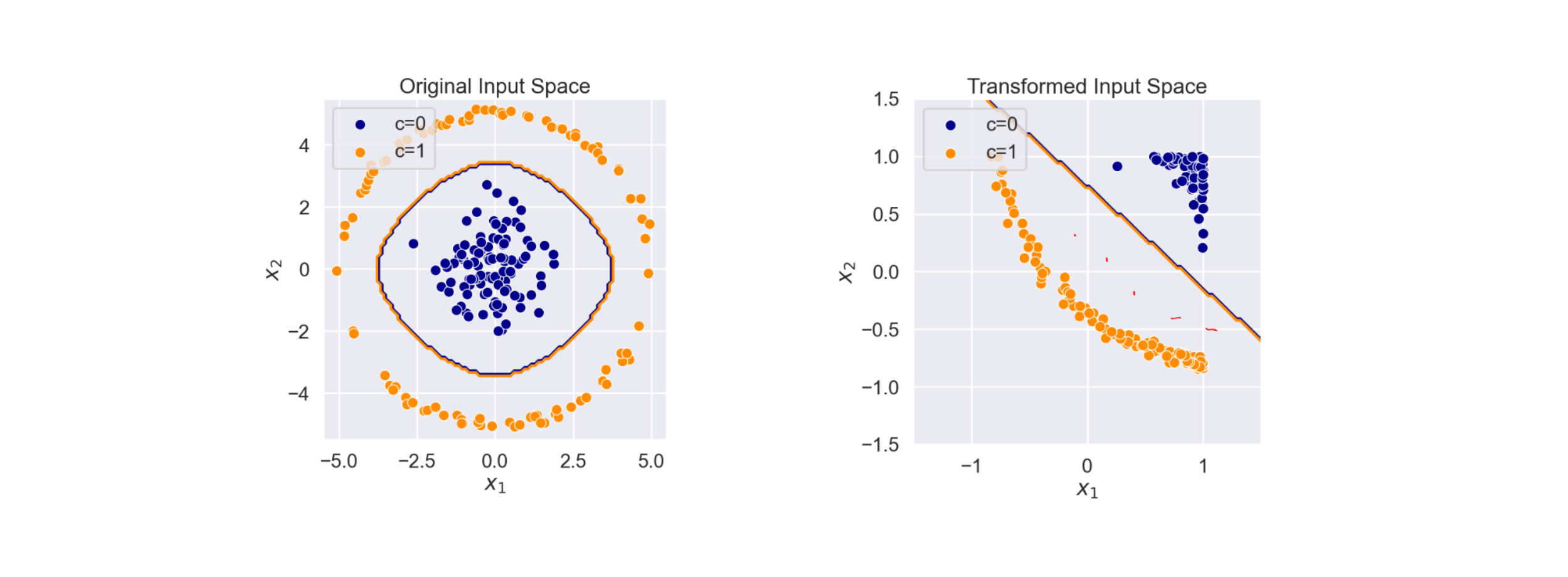
Transform input features
Given $x \in A$ i can transform it using $\phi(x)\in F$ called feature map. Es $\phi(x) = cos(x)$.
Ridge regression example
In ridge regression, we know $$w = \mathop{\arg \min}\limits_{w \in \mathbb{R}} \sum_{i=1}^N (y_i-w^Tx_i)^2 + \lambda |w|_2^2$$ Which has a closed form solution: $$w = (X^TX + \lambda I)^{-1}X^Ty$$
Using a feature map: $$w = \mathop{\arg \min}\limits_{w \in \mathbb{R}} \sum_{i=1}^N (y_i-w^T\phi(x_i))^2 + \lambda |w|_2^2$$ Which has a closed form solution: $$w = (\Phi^T\Phi + \lambda I)^{-1}\Phi^Ty$$ Where $$\Phi = [\phi (x_1), \phi (x_2), …, \phi (x_N)]^T$$.
Altough we have a closed form, calculating $\Phi^T\Phi$ might be difficult. Let’s try to write the dual of ridge regression:
$$e = \begin{bmatrix} y_1 - w^T\phi(x_1) \cr \vdots \cr y_N - w^T\phi(x_N)\end{bmatrix} = Y- \Phi W$$ Note how $e^Te = \sum_{i=1}^N (y_i- \phi(x))^2$
The optimization problem becomes: $$\mathop{\min}\limits_{w, e} \frac{1}{2}e^Te + \frac{1}{2}\lambda w^Tw$$ $$\text{subject to } e = Y - \Phi W$$ Solving this problem we get: $$y = w^{*T}\phi(x) = (\Phi^T\phi(x))^T(\Phi \Phi^T + \lambda I)^{-1} y$$ Where, for the kernel trick, both $\Phi \Phi^T$ and $\Phi^T\phi(x)$ does not depend on $\Phi$.
This is because the matrix $\Phi \Phi^T \in \mathbb{R}^{N \times N}$ is a GRAM matrix whose antries are $k_{ij} = < \phi(x_i), \phi(x_j)>$ For the mercer theorem $$k_{ij} = <\phi(x_i), \phi(x_j)> = k (x_i, x_j)$$ where $k$ is a valid kernel. For example (gaussian kernel) $k(a,b) = exp \set{- \frac{||a-b||^2}{2\sigma^2}}$
Non linear models
K-NN (K-nearest Neighbour)
Decision Trees
Multi layer perceptron (MLP)
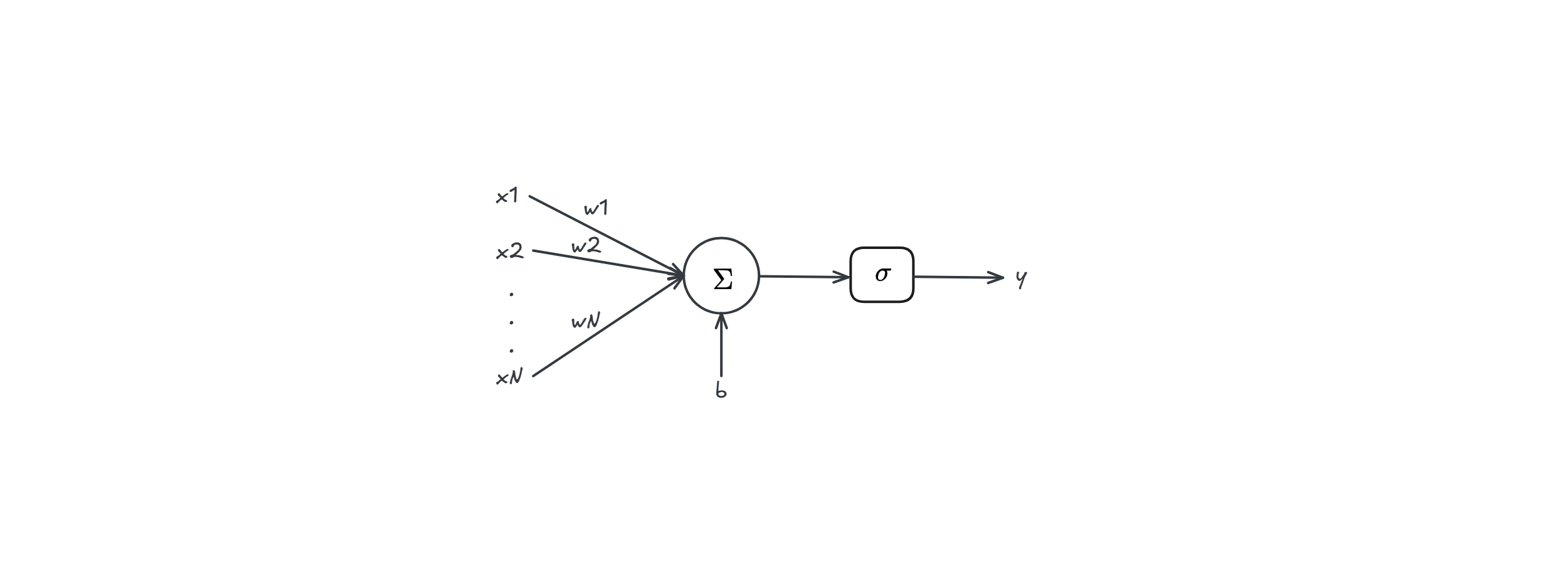
In perceptron we used $$y = sign(w^Tx+b)$$ A neuron is $$y = \sigma(w^Tx + b)$$ Where $\sigma$ is a
- non linear function (composition of linear function is linear)
- differentiable function (for training purpose)
Layer
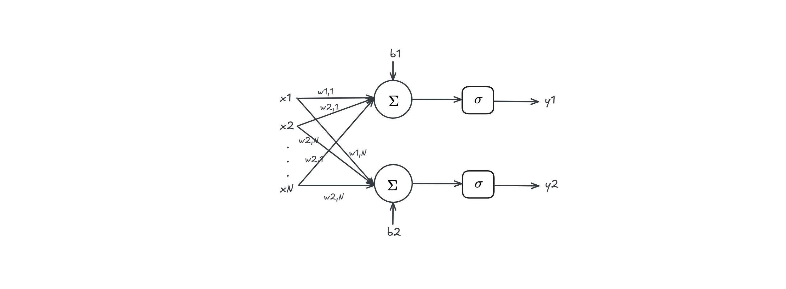
In this case we have
$$y = \begin{bmatrix} y_1 \cr y_2 \end{bmatrix} = \begin{bmatrix} \sigma(w_1^Tx + b_1) \cr \sigma(w_2^Tx + b_2) \end{bmatrix} = \sigma \Big(\begin{bmatrix} w_1^Tx + b_1 \cr w_2^Tx + b_2\end{bmatrix} \Big) = \sigma \Big( \begin{bmatrix} w_1^T x \cr w_2^T x \end{bmatrix} + \begin{bmatrix} b_1 \cr b_2 \end{bmatrix} \Big) = \sigma(Wx + b)$$
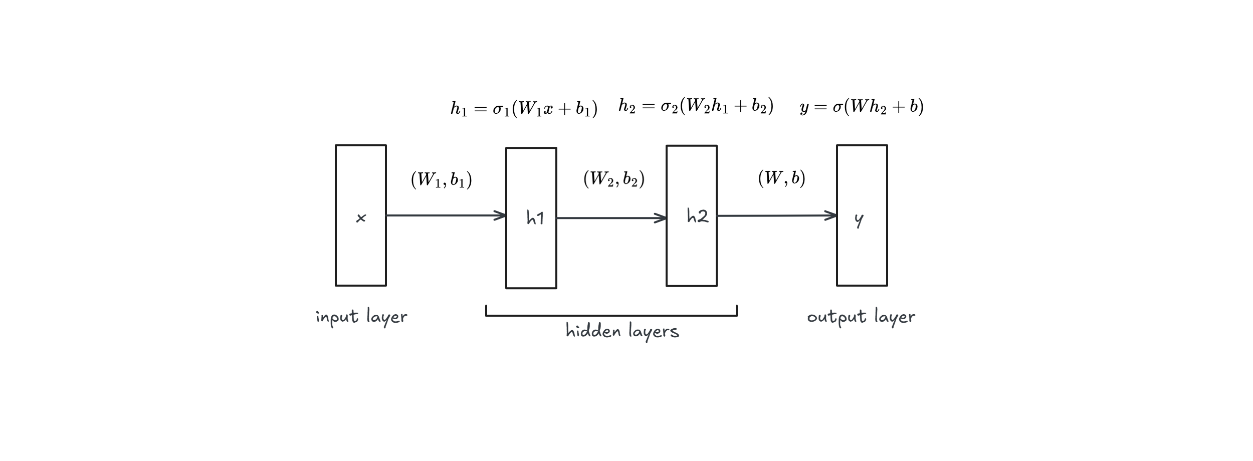
Multi-layer
In this case we have
- $y = \sigma(W h_2 + b)$
- $h_2 = \sigma_2(W_2 h_1 + b_2)$
- $h_1 = \sigma_1(W_1 x + b_1)$
Training a MLP
Suppose you have a dataset containing a single data point $D=\set{(x,y)}$. We take $L = MSE(h,D) = \frac{1}{2} (\tilde{y}-y)$
$$\frac{\partial L}{\partial q_i} = \frac{\partial L}{\partial y} \frac{\partial y}{\partial v} \frac{\partial v}{\partial q_i} = - (\tilde{y}- y)y(1-y)h_i$$ $$\frac{\partial L}{\partial c} = \frac{\partial L}{\partial y} \frac{\partial y}{\partial v} \frac{\partial v}{\partial c} = - (\tilde{y}- y)y(1-y)(1)$$ $$\frac{\partial L}{\partial w_{ij}} = \frac{\partial L}{\partial y} \frac{\partial y}{\partial v} \frac{\partial v}{\partial h_i} \frac{\partial h_i}{\partial u} \frac{\partial u}{\partial w_{ij}} = - (\tilde{y}- y)y(1-y)q_ih_i(1-h_i)x_i$$ $$\frac{\partial L}{\partial b_i} = \frac{\partial L}{\partial y} \frac{\partial y}{\partial v} \frac{\partial v}{\partial h_i} \frac{\partial h_i}{\partial u} \frac{\partial u}{\partial b_i} = - (\tilde{y}- y)y(1-y)q_ih_i(1-h_i)(1)$$
So while doing gradient descent, we will update parameters following the steepest descent i.e $-\frac{\partial L}{\partial \theta}$
Training a MLP for larger dataset
For larger dataset $D= \set{(x_1,y_1),…,(x_N,y_N)}$ and $$L = MSE(h,D) = \frac{1}{N} \sum_{i=1}^N (\tilde{y}-y)^2$$ But since we can write $$L = \frac{1}{N} \sum_{i=1}^{N} L_i$$ This impy that $$\frac{\partial L}{\partial \theta} = \frac{1}{N} \sum_{i=1}^N \frac{\partial L_i}{\partial \theta}$$ And we already know how to calculate $\frac{\partial L_i}{\partial \theta}$
Gradient descent
There are a few ways to do gradient descent, which is the process of minimizing $$L_{tr} = \frac{1}{N} \sum_{i=1}^N L(\tilde{y_i}, f_\theta(x_i))$$
- FULL-BATCH
- STOCHASTIC GRADIENT DESCENT
- Sequential mode
- mini-batch mode
Before explaining them in details let’s explore some background knowledge:
definition (descent direction): $p \in \mathbb{R}^n$ is a descent direction for $f$ in a point $x$ if $$\frac{\partial f}{\partial p} (x) = \overbrace{\nabla f(x)^T p}^{\in \mathbb{R}} < 0$$
steepest descent direction: if $\nabla f(x) \neq 0$ we have always a steepest descent direction: $$-\nabla f(x)$$
this is because $$\nabla f(x)^T p = ||\nabla f(x)|| ||p|| cos \theta = ||\nabla f(x)|| \overbrace{cos \theta}^{\text{minimum when } \theta = -1 }$$
Full-batch
We follow the direction of maximum descent, i.e $\frac{\partial L_{tr}}{\partial \theta}$
- $\forall epochs$
- reset gradients $\frac{\partial L}{\partial \theta}$
- $\forall (x_i,\tilde{y_i}) \in D_{tr}$
- $y_i = MLP_\theta (x_i)$
- compute $L(\tilde{y_i},y_i)$
- compute $\frac{\partial L(\tilde{y_i},y_i)}{\partial \theta_j}$
- accumulate $\frac{\partial L}{\partial \theta_j} = \frac{\partial L}{\partial \theta_j} + \frac{\partial L(\tilde{y_i},y_i)}{\partial \theta_j}$
- update all parameters $\theta$
Stochastic gradient descent
We approximate the direction of maximum descent $$\frac{\partial L_{tr}}{\partial \theta} \approx \frac{\partial L_i}{\partial \theta}$$
- $\forall epochs$
- $\forall (x_i,\tilde{y_i}) \in D_{tr}$
- $y_i = MLP_\theta (x_i)$
- compute $L(\tilde{y_i},y_i)$
- compute $\frac{\partial L(\tilde{y_i},y_i)}{\partial \theta_j}$
- update all parameters $\theta$
- $\forall (x_i,\tilde{y_i}) \in D_{tr}$
Mini Batch mode
We approximate the direction of maximum descent $$\frac{\partial L_{tr}}{\partial \theta} \approx \frac{1}{|BATCH|} \sum_{i \in BATCH}\frac{\partial L_i}{\partial \theta}$$
- $\forall epochs$
- split $D_{tr}$ in batches of size $|BATCH|$
- $\forall \text{ batch } B$
- reset gradients $\frac{\partial L}{\partial \theta}$
- $\forall (x_i,\tilde{y_i}) \in B$
- $y_i = MLP_\theta (x_i)$
- compute $L(\tilde{y_i},y_i)$
- compute $\frac{\partial L(\tilde{y_i},y_i)}{\partial \theta_j}$
- accumulate $\frac{\partial L}{\partial \theta_j} = \frac{\partial L}{\partial \theta_j} + \frac{\partial L(\tilde{y_i},y_i)}{\partial \theta_j}$
- update all parameters $\theta$
Conclusion
When we said “update all parameters $\theta$” what we mean is taking small steps in the calculated direction, there are many ways optimizer do this, the most naive way is basic line search:
$$\theta^{new} = \theta^{old} - \alpha \frac{\partial L}{\partial \theta}$$
MLP Hyperparameters & how to choose them
There are many, many hyperparameters in MLP:
- number of layers
- number of neurons in each layer
- activation functions: There are many, here is a little list
- sigmoid $$sigmoid(x) = \sigma(x) = \frac{1}{1+ e^{-x}}$$
- hyperbolic tangent $$tanh(x) = \frac{1-e^{2x}}{1+ e^{-2x}}$$
- ReLu (Rectified Linear Unit) $$ReLu(x) = max(0,x)$$
- Leaky ReLu $$LeakyReLu(x) = max(-\alpha x, x) , \alpha > 0$$
- output functions
- Sign function $$sign(x) = 1 \text{ if } x > 0 \text{ else } -1$$
- Identity function $$identity(x) = x$$
- softmax function $$softmax(x)_i = \frac{e^{x_i}}{\sum_j e^{x_j}}$$
- loss function
- MSE (Mean Squared Error) $$MSE = \frac{1}{N} \sum_{i=1}^N (\tilde{y_i} - f_\theta(x))^2$$
- MAE (Mean Absolute Error) $$MAE = \frac{1}{N} \sum_{i=1}^N |\tilde{y_i} - f_\theta(x)|$$
- Cross Entropy $$CROSSENTROPY = \frac{1}{N} \sum_{i=1}^N \sum_{k=1}^{K} y_{ik} log(p_{ik})$$
- learning rate
- … many more

The choice of the loss and the output function are strictly related.
Regression Task: One neuron with identity function + MSE/MAE loss
Binary Classification Task: One neuron with logistic sigmoid function + Binary CE loss
Multi-class classification Task: One neuron for each class with softmax function + CE loss
Regularising MLP
It can be possible to regularise a MLP in order to avoid overfitting
Penalisation
$$J^{’}(D_{tr}, \theta) = \overbrace{L(D_{tr}, \theta)}^{J(D_{tr},\theta)} + \lambda R(\cdot)$$
Where: $$R(\cdot) = \overbrace{R(\theta)}^{\text{penality on parameters}} + \overbrace{R(Z)}^{\text{penality on activations}} = ||\theta||_2^2 + ||Z||_2^2$$
If we differentiate $J’(D_{tr},\theta)$: $$\nabla_\theta J’(D_{tr}, \theta) = \nabla J(D_{tr}, \theta) + 2 \lambda \theta$$ We get that $$\theta^{new} = \theta^{old} - \alpha \big(\nabla_{\theta^{old}}J’(D_{tr}, \theta^{old}) \big)$$ $$= \theta^{old} - \alpha \big(\nabla_{\theta^{old}}J(D_{tr}, \theta^{old}) + 2 \lambda \theta^{old} = \theta^{old} \overbrace{(1 - 2 \alpha \lambda )}^{\text{weight decay}} - \alpha \nabla_{\theta^{old}} J(D_{tr}, \theta^{old})$$
Notice how if $\lambda = 1$, the whole weight decay term is $1$, so it is just standard weight update.
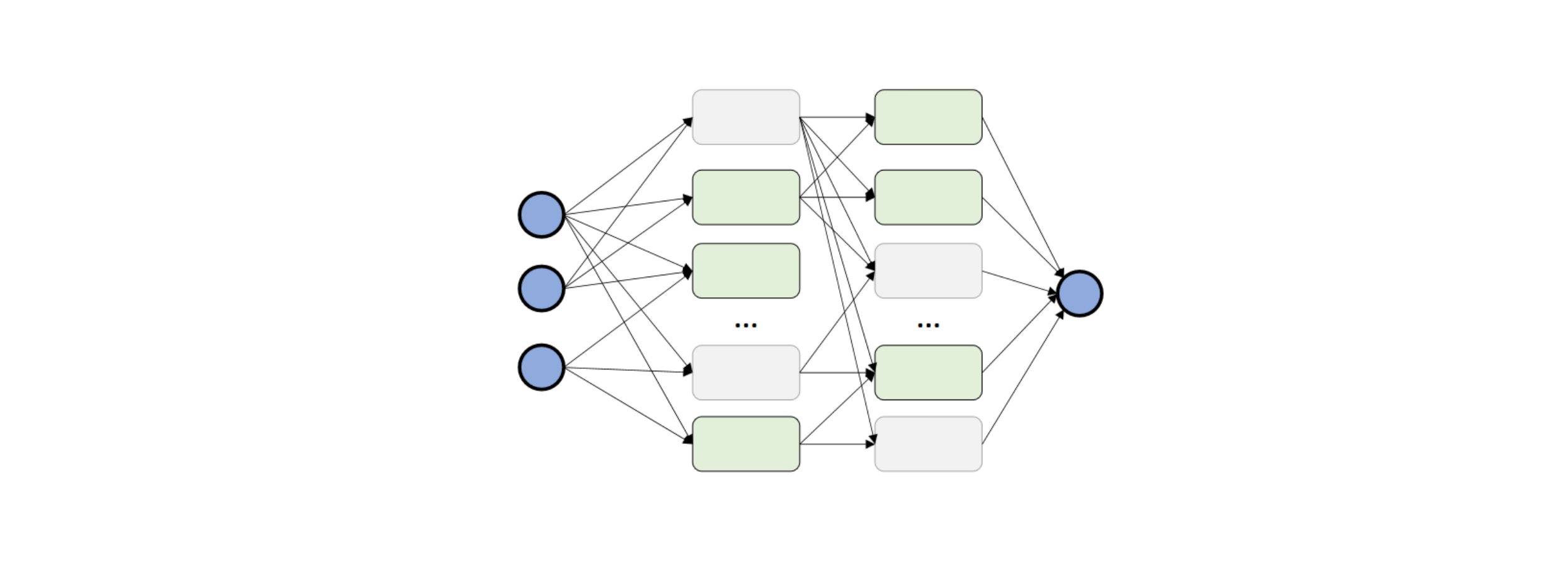
Dropout regularisation
We randomly disconnect units from the network during training and change the disconnected units at each minibatch
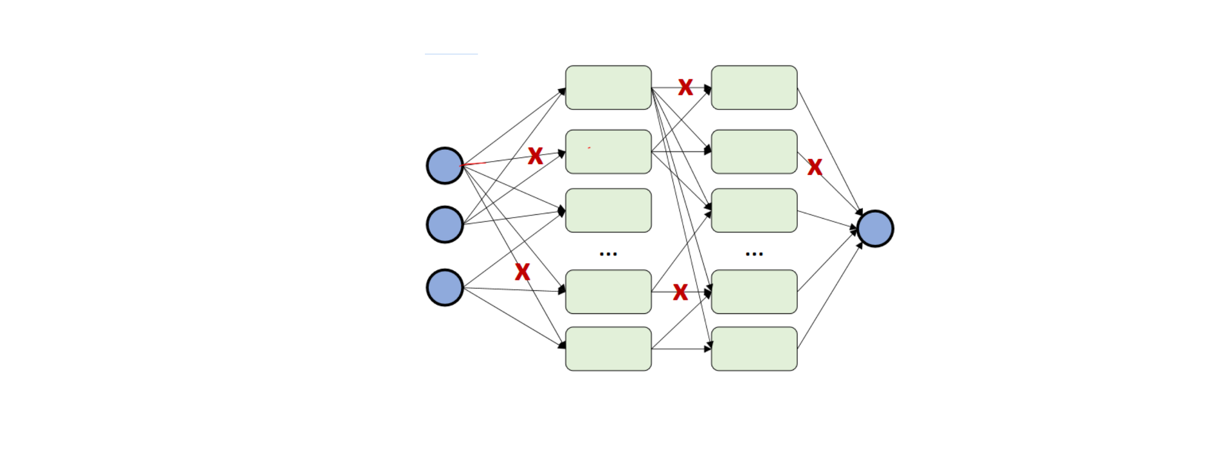
You can also drop single connections (dropconnect)
Early stopping
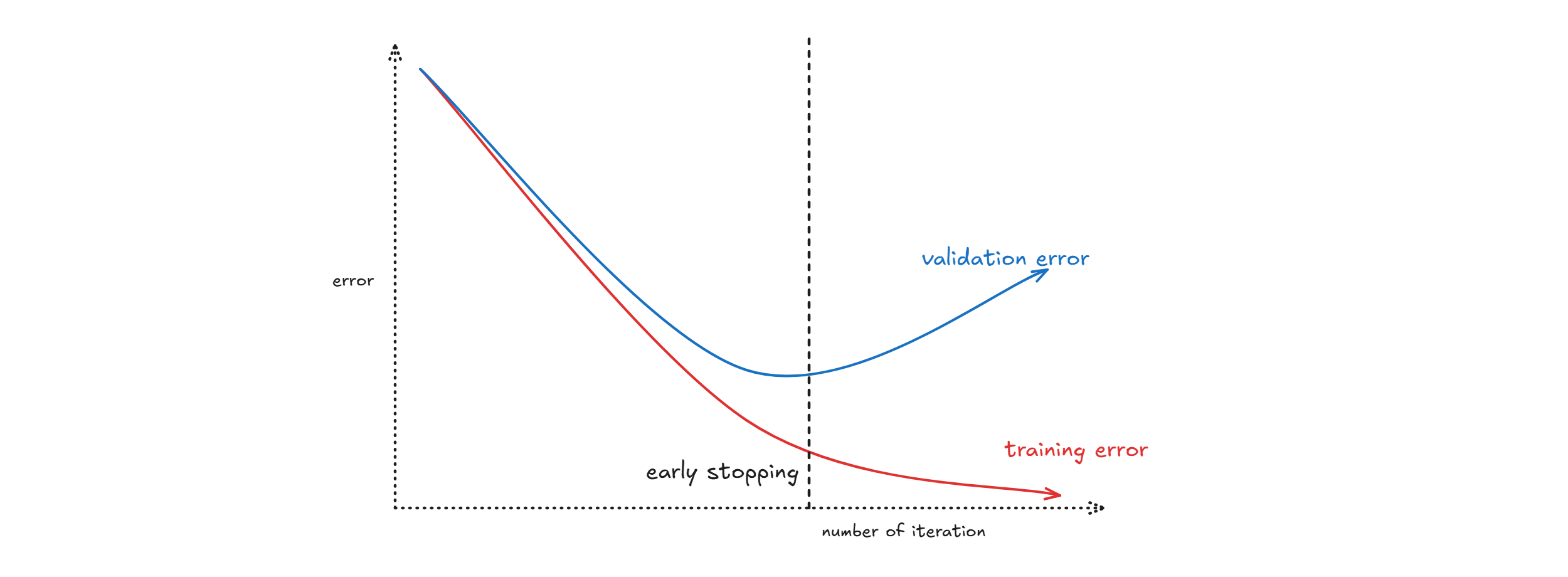
Estimate the generalisation error on the val. set after every epoch and maintain weights for best performing network on the validation set and stop training when error increases beyond this. Run the network for some epochs before deciding to stop (patience).
Deep Learning for Sequences
A sequence is
$$X = (x_1,…,x_T), x_1 \prec x_2 … \prec x_T$$
Naive: with Multi Layer Perceptron (MLP)
We can use a MLP to do that but it is impractical:
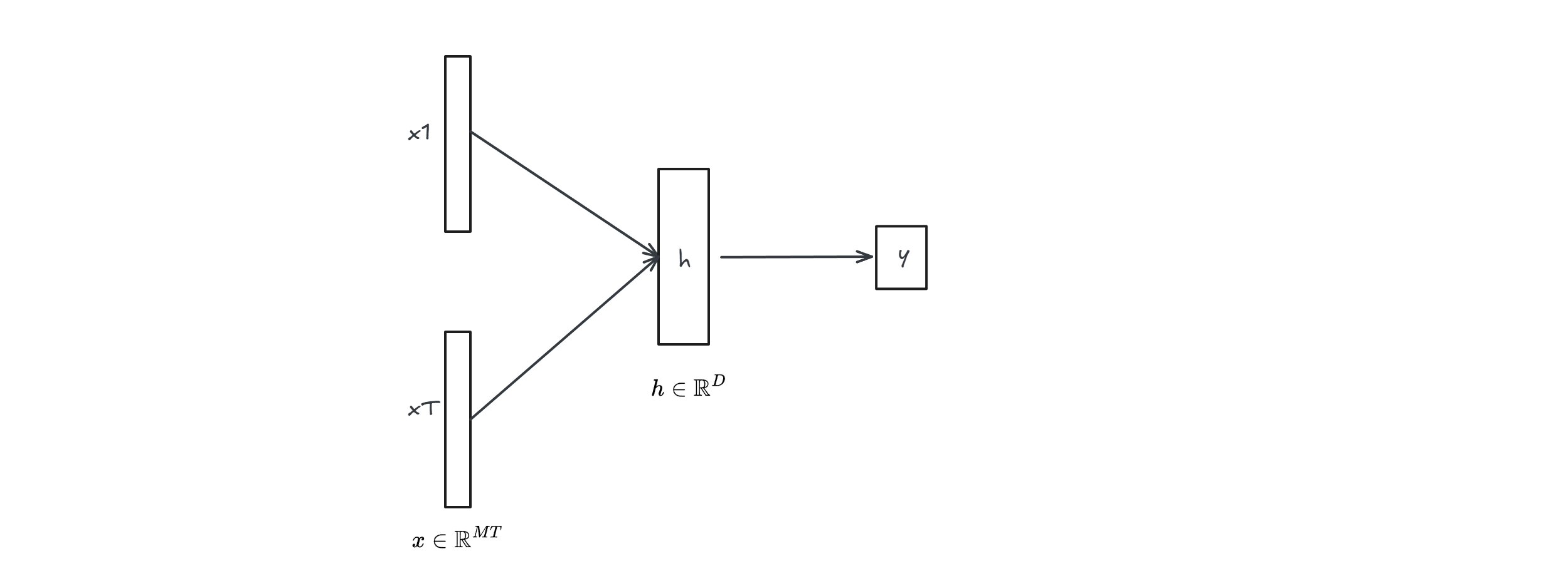
Because if $x \in \mathbb{R}^{MT}, h \in \mathbb{R}^D$ then $$W \in \mathbb{R}^{MT \times D}$$
So the number of parameters depends on the sequence length $T$, very bad ;(
There is also another problem, what if we want to classify a sequence of length $T’>T$? we should trim the new sequence while losing information. Note that if we want to classify a sequence of length $T’ < T$ we can just put the trailing features to 0 with no problem.
Recurrent Neural Network (RNN)
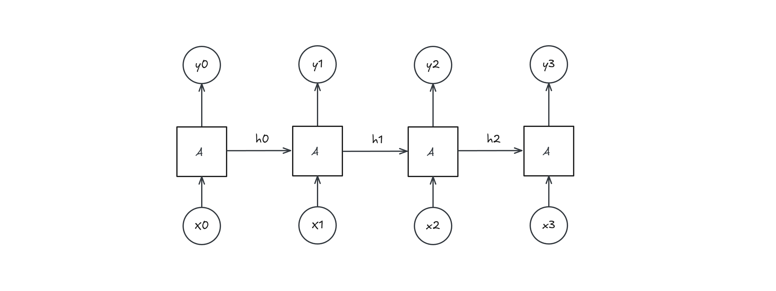
Idea: for each time step we keep a hidden state $h_t$ which can be used to produce $y_t$

The state is passed between all time steps: this is how the network looks when unrolled (for a sequence of length 4):
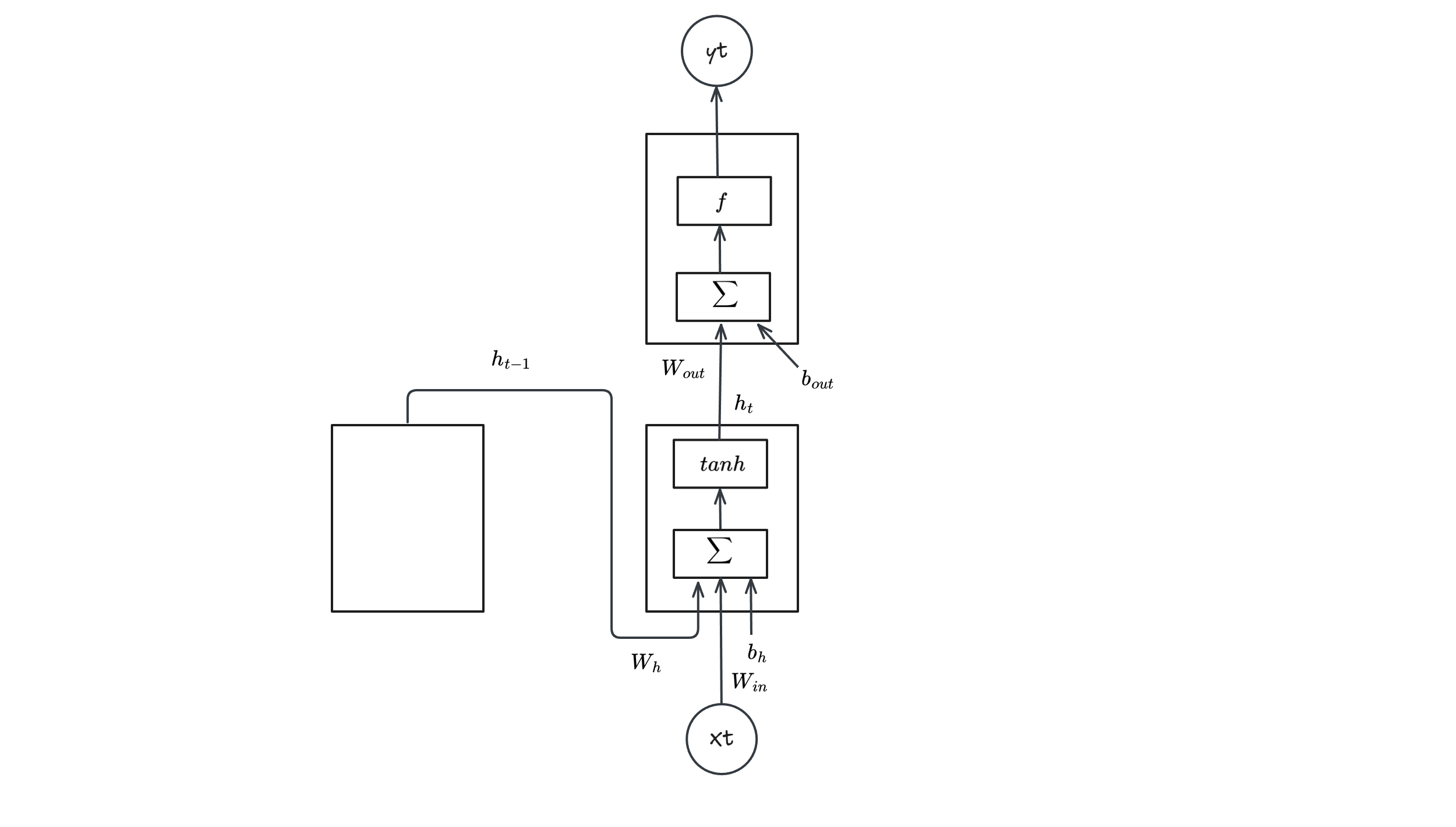
Going into details a RNN can be described with the following mathematical equations:
- $h_t = tanh(g_t)$
- $g_t = W_hh_{t-1} + W_{in}x_t + b_h$
- $y_t = f(W_{out}h_t + b_{out})$
RNN problems
RNN have mainly 2 problems:
- Learning long term dependencies is difficult
imagine a network with 100 steps:
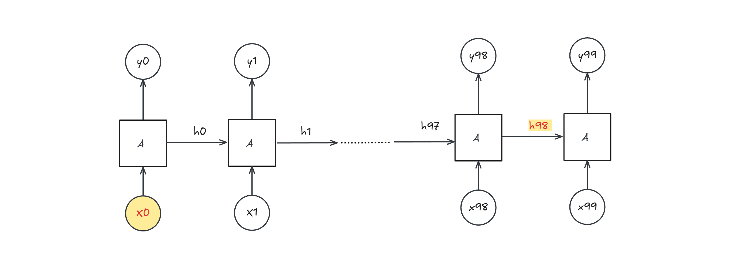
$h_{98}$ has a fixed size representation and contains very little information about $x_0$.
- Vanishing/Exploding gradients
Let’s write the backprop formula
$$L = \sum_{t=1}^T L_t(y_t, \tilde{y}_t)$$
$$\frac{\partial L_t}{\partial w} = \frac{\partial L_t}{\partial y_t} \frac{\partial y_t}{\partial h_t} \frac{\partial h_t}{\partial w}$$
and since $h_t(w, h_{t-1}(w, …)$ we can write
$$\frac{\partial h_t}{\partial w} = \frac{\partial h_t}{\partial w} + \frac{\partial h_t}{\partial h_{t-1}} \frac{\partial h_{t-1}}{\partial{w}}$$
Now expanding recursively on $\frac{\partial h_{t-1}}{\partial{w}}$
$$ = \frac{\partial h_t}{\partial w} + \frac{\partial h_t}{\partial h_{t-1}} (\frac{\partial h_{t-1}}{\partial w} + \frac{\partial h_{t-1}}{\partial h_{t-2}} \frac{\partial h_{t-2}}{\partial w})$$
$$= \frac{\partial h_t}{\partial w} + \frac{\partial h_t}{\partial h_{t-1}} \frac{\partial h_{t-1}}{\partial w} + \frac{\partial h_t}{\partial h_{t-1}} \frac{\partial h_{t-1}}{\partial h_{t-2}} \frac{\partial h_{t-2}}{\partial w}$$
$$…$$ $$ = \sum \Big( \prod \frac{\partial h_i}{\partial h_{i-1}} \Big) \frac{\partial h_i}{\partial w}$$
And since
$$\frac{\partial h_i}{\partial h_{i-1}} = \frac{\partial h_i}{\partial g_i} \overbrace{\frac{g_i}{h_{i-1}}}^{w}$$
$$\rightarrow \frac{\partial h_t}{\partial w} \approx \sum (\prod w)$$
So if $|w| > 1$ gradient is going to explode, if $|w| < 1$ then gradient is going to vanish.
Long Short Term Memory (LSTM)
To solve RNN problems, Long Short Term Memory (LSTM) architecture has been proposed:
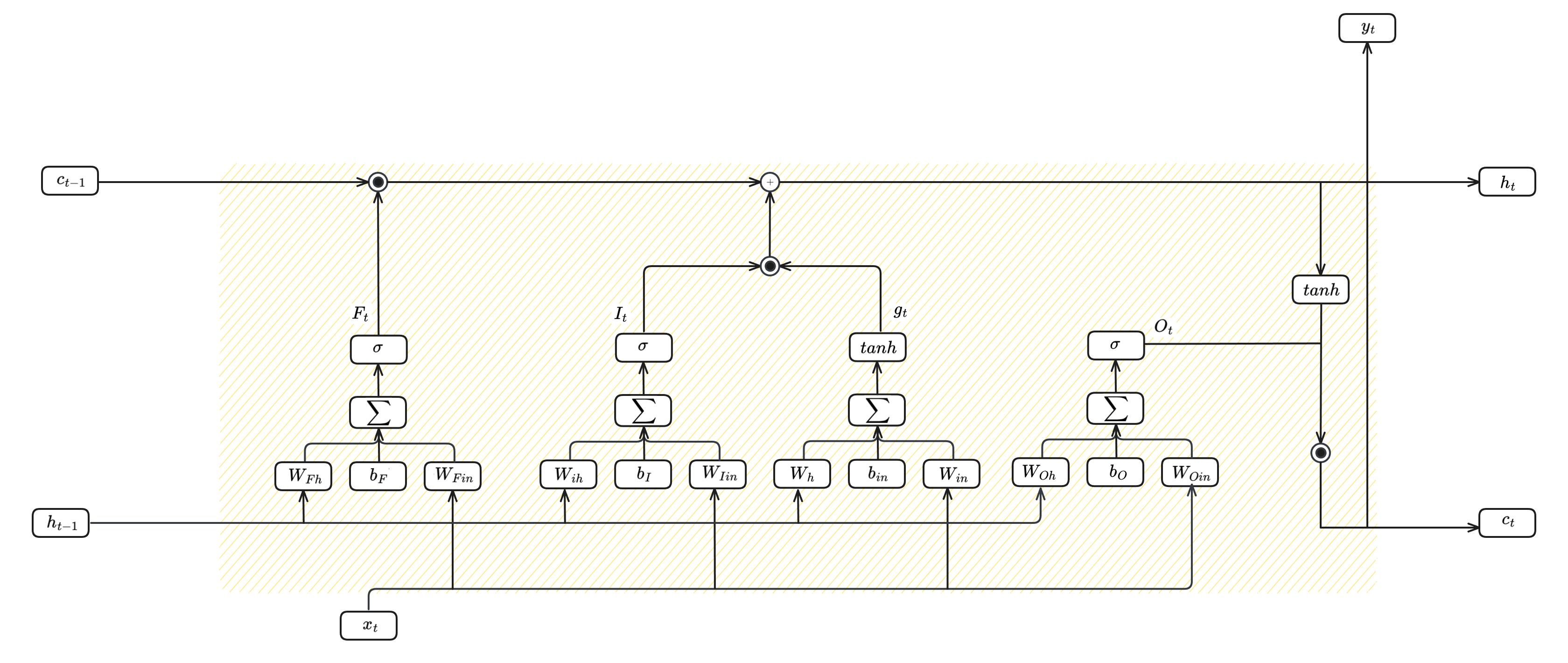
It can also be described by the following equations:
- $F_t = \sigma(W_{Fh}h_{t-1} + W_{Fin}x_t + b_F)$
- $I_t = \sigma(W_{Ih}h_{t-1} + W_{Iin}x_t + b_I)$
- $g_t = tanh(W_{hg}h_{t-1}+ W_{in}x_t + b_h)$
- $c_t=F_t \bigodot c_{t-1} + I_t \bigodot g_t$
- $O_t = \sigma(W_{Oh}h_{t-1} + W_{Oin}x_t + b_O)$
- $h_t = O_t \bigodot tanh(c_t)$
The one above is a single LSTM cell, they can be stacked together and form a lstm layer.
NLP
core NLP steps and techniques
- Tokenization:
Definition: Splitting text into smaller units (tokens), typically words or punctuation.
Example:
Input: “The quick brown fox jumps over the lazy dog.”
Output: [“The”, “quick”, “brown”, “fox”, “jumps”, “over”, “the”, “lazy”, “dog”, “.”]
- Lemmatization/Stemming:
Definition: Reducing words to their base or root form.
Lemmatization: Uses a dictionary to find the correct base form (lemma).
Stemming: Removes suffixes, often resulting in non-words.
Example:
Input: “running”, “runs”, “ran”
Lemmatization Output: “run”, “run”, “run”
Stemming Output: “run”, “run”, “ran”
- Bag of Words (BOW):
Definition: Represents text as a collection of words and their frequencies, disregarding grammar and order.
Example:
Documents:
D1: “The cat sat on the mat.”
D2: “The dog sat on the rug.”
Vocabulary: [“the”, “cat”, “sat”, “on”, “mat”, “dog”, “rug”]
BOW Representation:
| Word | D1 | D2 |
|---|---|---|
| the | 2 | 1 |
| cat | 1 | 0 |
| sat | 1 | 1 |
| on | 1 | 1 |
| mat | 1 | 0 |
| dog | 0 | 1 |
| rug | 0 | 1 |
- One-Hot Encoding:
Definition: Creates a binary vector for each word, indicating its presence in a document or sentence.
Example:
Vocabulary: [“cat”, “dog”, “mat”]
Word: “cat”, One-Hot Vector: [1, 0, 0]
Word: “dog”, One-Hot Vector: [0, 1, 0]
Word: “mat”, One-Hot Vector: [0, 0, 1]
- TF-IDF (Term Frequency-Inverse Document Frequency):
Definition: Assigns weights to words based on their frequency in a document and their rarity across the corpus.
- Word2Vec:
Definition: Creates vector representations of words that capture semantic relationships. Words with similar meanings have similar vectors.
For example Word2Vec would represent “king” and “queen” as vectors that are close in vector space. It’s a complex process, and the output is a set of vectors, not a simple table.
- GloVe (Global Vectors for Word Representation):
Definition: Similar to Word2Vec, GloVe creates word vectors based on word co-occurrence statistics in a corpus.
Language Modelling (LM)
Given a sequence $\set{x_1,…,x_T}$ we want to know $P(x_{T+1}|x_1,…,x_T)$
N-grams model
We assume only last N word counts
For example with $N=4$ $$P(x_t | x_{t-1}, x_{t-2},x_{t-3},x_{t-4}) \approx \frac{\text{#}\set{x_t,x_{t-1},x_{t-2},x_{t-3},x_{t-4}}}{\text{#} \set{x_{t-1},x_{t-2},x_{t-3},x_{t-4}}}$$
Example:
Suppose we are learning a 4-gram Language Model:
$$\text{as the proctor started the clock, the students opened their ____}$$
Suppose
- “students opened their” occurred 1000 times
- “students opened their books” occurred 400 times
- “students opened their exams” occurred 100 times
We can approximate
$$P(\text{books}| \text{students, opened, their}) \approx \frac{\text{#} \text{students, opened, their, books}}{\text{# students, opened, their}} = \frac{400}{1000} = 0.4$$
$$P(\text{exams}| \text{students, opened, their}) \approx \frac{\text{#} \text{students, opened, their, exams}}{\text{# students, opened, their}} = \frac{100}{1000} = 0.1$$
Indeed, “exams” is the right answer!
Window Based NN
You can imagine using a NN to do this task, however the problem is that the parameters number is tightly coupled with the sequence length…
RNN
A better way is using RNN with $f = softmax$
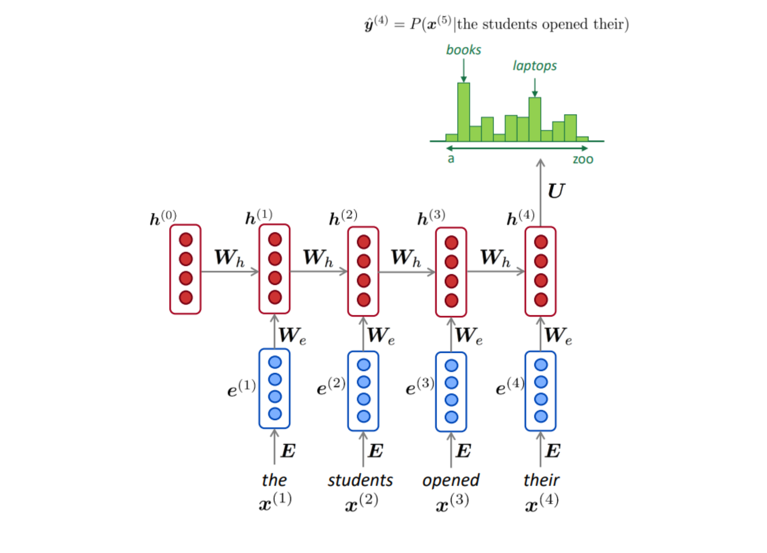
To train such model (teacher forcing):
given a corpus $\set{x_1,…,x_T}$
- $\forall t=1,…,T$
- compute $$P(x_t|x_{t-1},…,x_1)$$
- compute $$L_t = CE(\text{predicted prob distrib, true prob distrib})$$
Neural Machine Translation (NMT)
is a seq-to-seq problem where we have
$$\text{x} \rightarrow \text{encoder} \rightarrow \text{z} \rightarrow \text{decoder} \rightarrow \text{y}$$

This kind of architecture has a problem: there is a information bottleneck. All the information is encoded in a fixed size hidden state $h$. You can think of a solution where you concatenate $h$ with every state of the decoder, but this will lead again to information bottleneck. We need to explore other architectures:
Attention
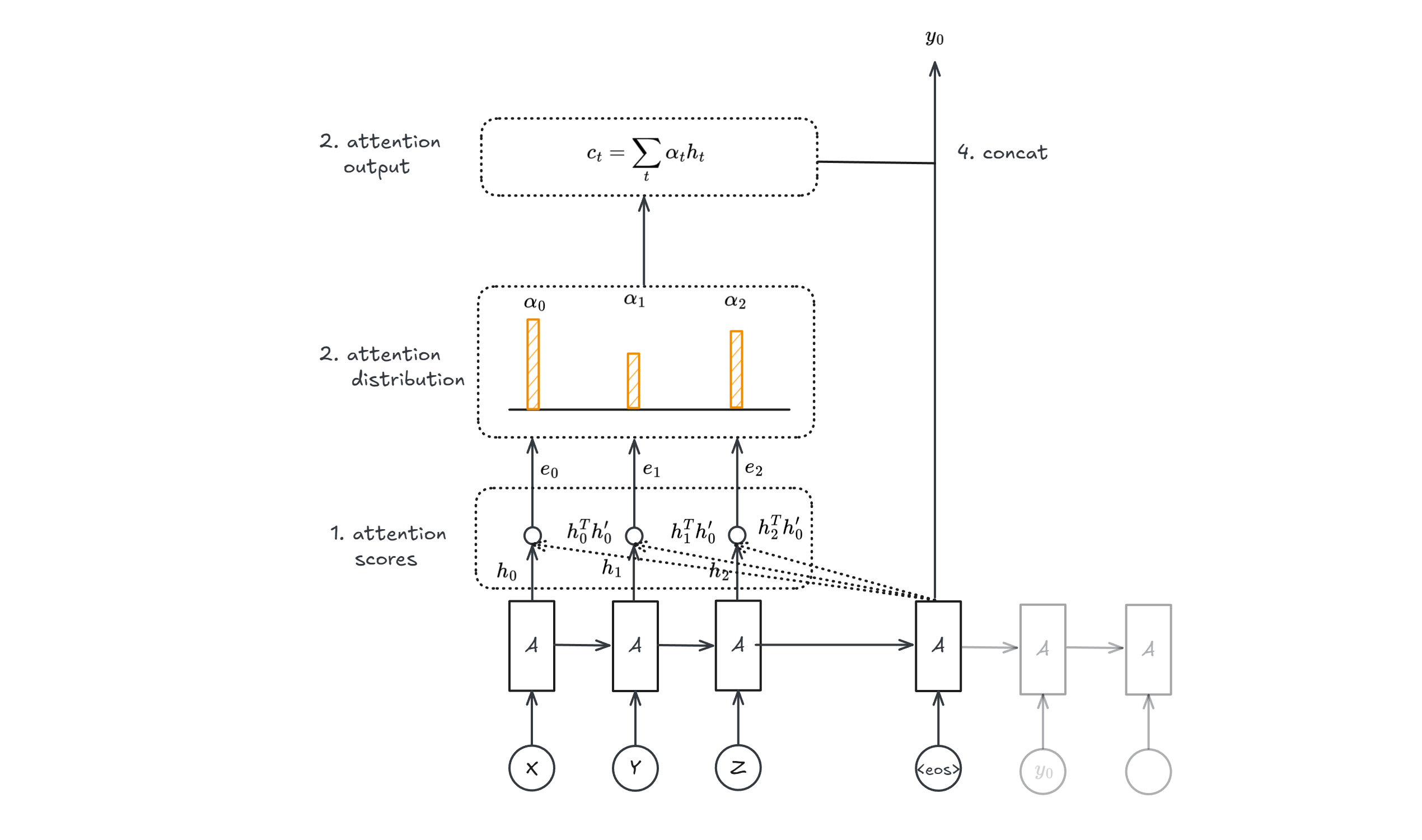
Where
- Attention Scores: $e_i = h_i^T h_i’ \forall i$ is a similarity measure
- Attention Distribution: it’s a softmax to all attention scores
- Weighted Sum: all $\alpha_t$ are the probabilities of softmax
- Concatenation: the attention output gets concatenated with decoder hidden state
Attention is a general mechanism:
$$Attention(q, (k_i, v_i)) = \sum_{i=1}^N softmax(q^T k_i) v_i$$
The image above shows only one step, the second one would be the following:
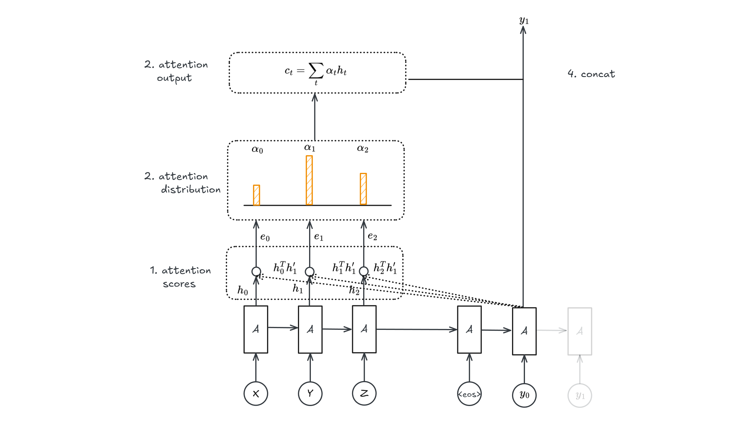
Deep Learning for Unsupervised Learning
In a supervised learning task, the DL model learns from an input-output pair $(x,y)$.
In an unsupervised learning task,the DL model learns only from an input.
Some unsupervised tasks are:
- clustering
- anomaly detection
- dimensionality reduction
- generative tasks
- …
Clustering
K-Means
Algorithm
- Select $k$ points as the initial centroids
- repeat
- Form $K$ clusters by assigning all points to the closest centroid
- Recompute the centroid of each cluster
- until the centroids don’t change
The complexity of the algorithm is
$$O(\overbrace{n}^{\text{ #point }} \overbrace{K}^{\text{ #cluster }} \overbrace{I}^{\text{ #iteration }} \overbrace{d}^{\text{ #dimension }})$$
To evaluate K-means algorithm it is possible to use the $SSE$ metric:
$$SSE = \sum_{i=1}^{K} \sum_{x \in c_i} dist(x_i,m_i)^2$$
To minimize this metric.
- If we use the euclidean distance as a distance function ($dist(a,b) = (a-b)^2$) then we have to choose $$c_i = \frac{1}{|C_i|}\sum_{x \in C_i} x$$
proof:
$$\frac{\partial}{\partial c_k} SSE = 0 = \frac{\partial}{\partial c_k} \sum_{i=1}^{K}\sum_{x \in C_i} (x-c_i)^2$$ $$=\sum_{i=1}^{K} \sum_{x \in C_i} \frac{\partial}{\partial c_k} (x-c_i)^2 = \sum_{x \in c_k} 2(c_k-x)$$
$$\rightarrow c_k = \frac{1}{|C_k|} \sum_{x \in C_k} x$$
Dimensionality reduction
Auto-Encoders
We can use a auto-encoder model to do dimensionality reduction. An auto-encoder is a model composed of 2 parts: one encoder ($f$) and one decoder ($g$).
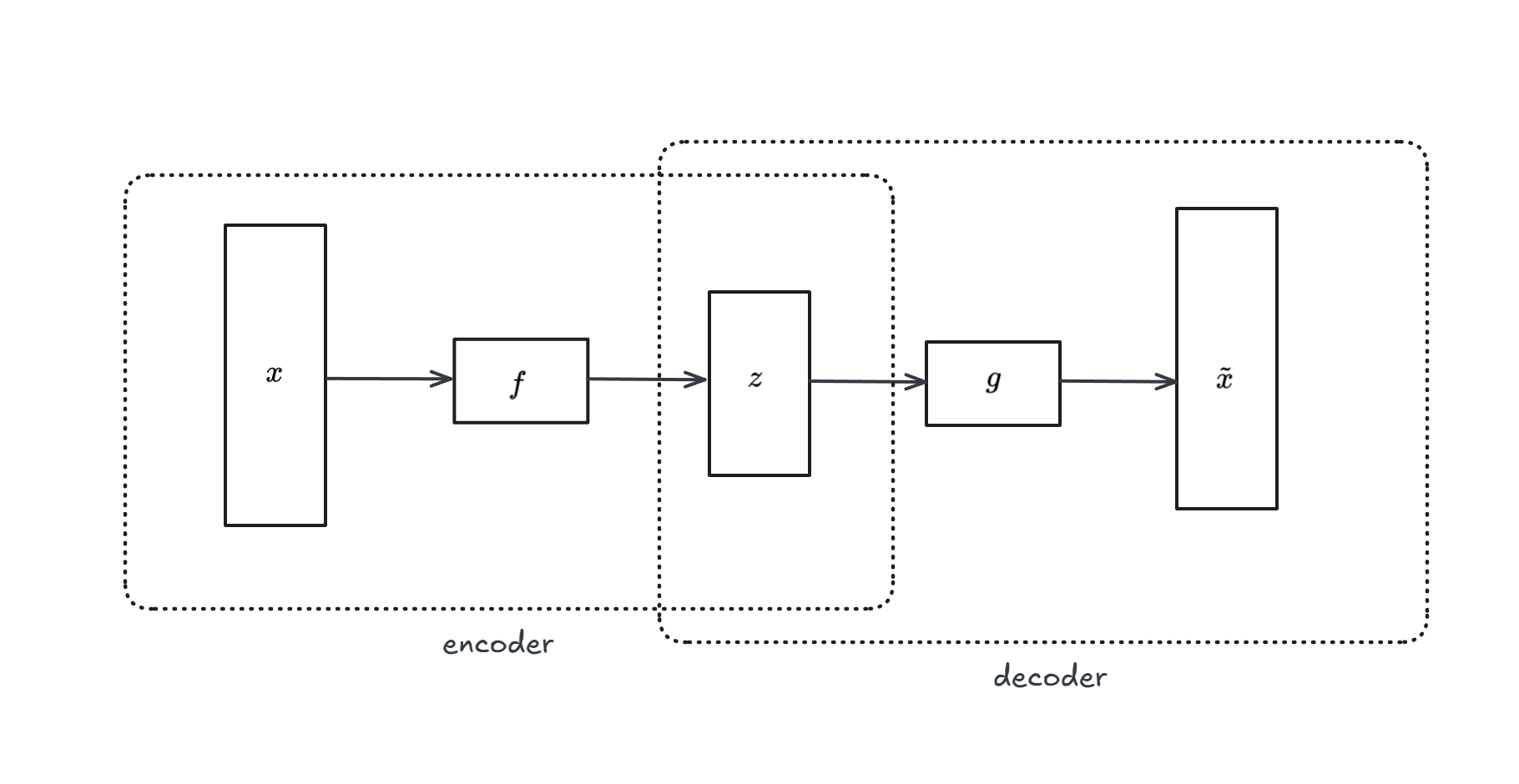
$f$ and $g$ can be any DL models, like MLP, CNN, LSTM…
The objective function is the recostruction, i.e we find $f$ and $g$ that minimises $L(x,\tilde{x})$.
Once the model is learned, we can take the latent vector ($z$) as a reduced dimensionality rapresentation of the input (we detach the decoder part).
Generative models
The onbjective of generative models is: given training data, learn a (deep) neural network that can generate new samples from (an approximation of) the data distribution
Variational Auto-Encoder (VAE)
One can think to take an auto-encoder architecture, and simply sample from the latent space ($z$) to generate new samples. The problem with this approach is that the latent space is not organized.
We then need to organize it:
interpreting $f$ and $g$ as probability distribution, we can write
$$P_f(z|x) = \frac{P(x|z)P(z)}{P(x)} = \frac{P(x|z)P(z)}{\int P(x|z)P(z) dz}$$
The integral is intractable, so we approximate $P_f(z|x)$ with a known distribution $q$:
$$P_f(z|x) \approx q(z|x) \sim \mathcal{N}(\mu(x), \sigma(x))$$
To make those probability distribution as close as possible we need to minimize a similarity measure, i.e find:
$$q* = argmin_{q \in Q} KL(p||q)$$
A VAE network can be visualized as follows:
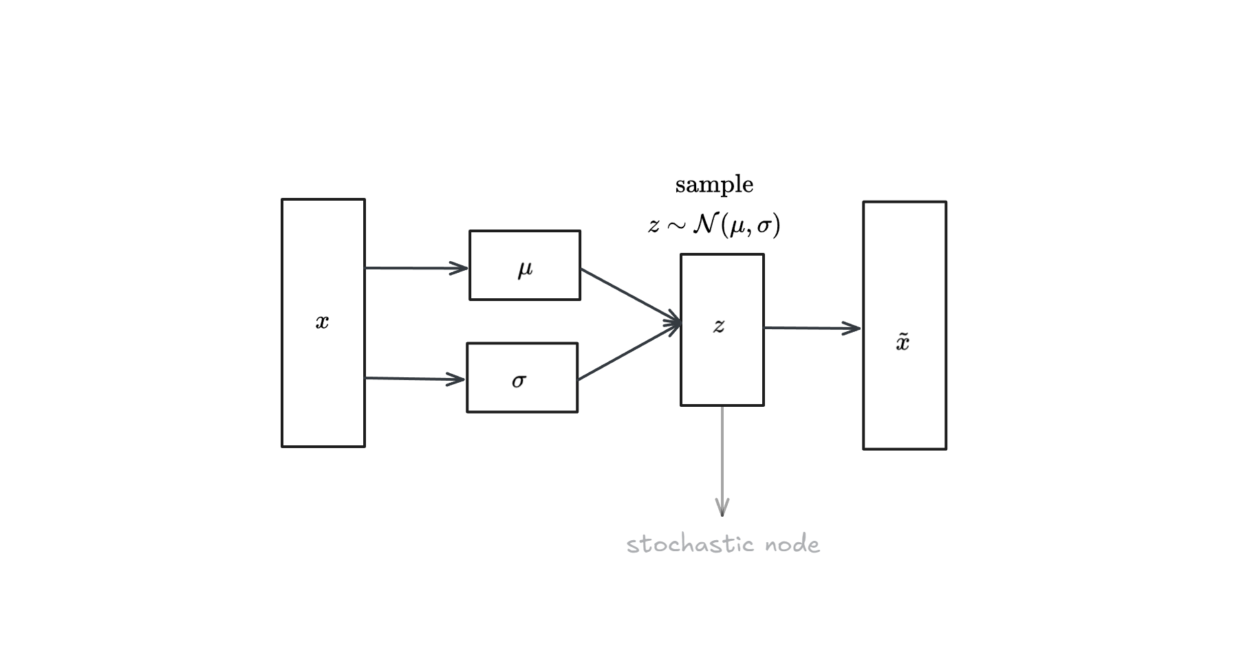
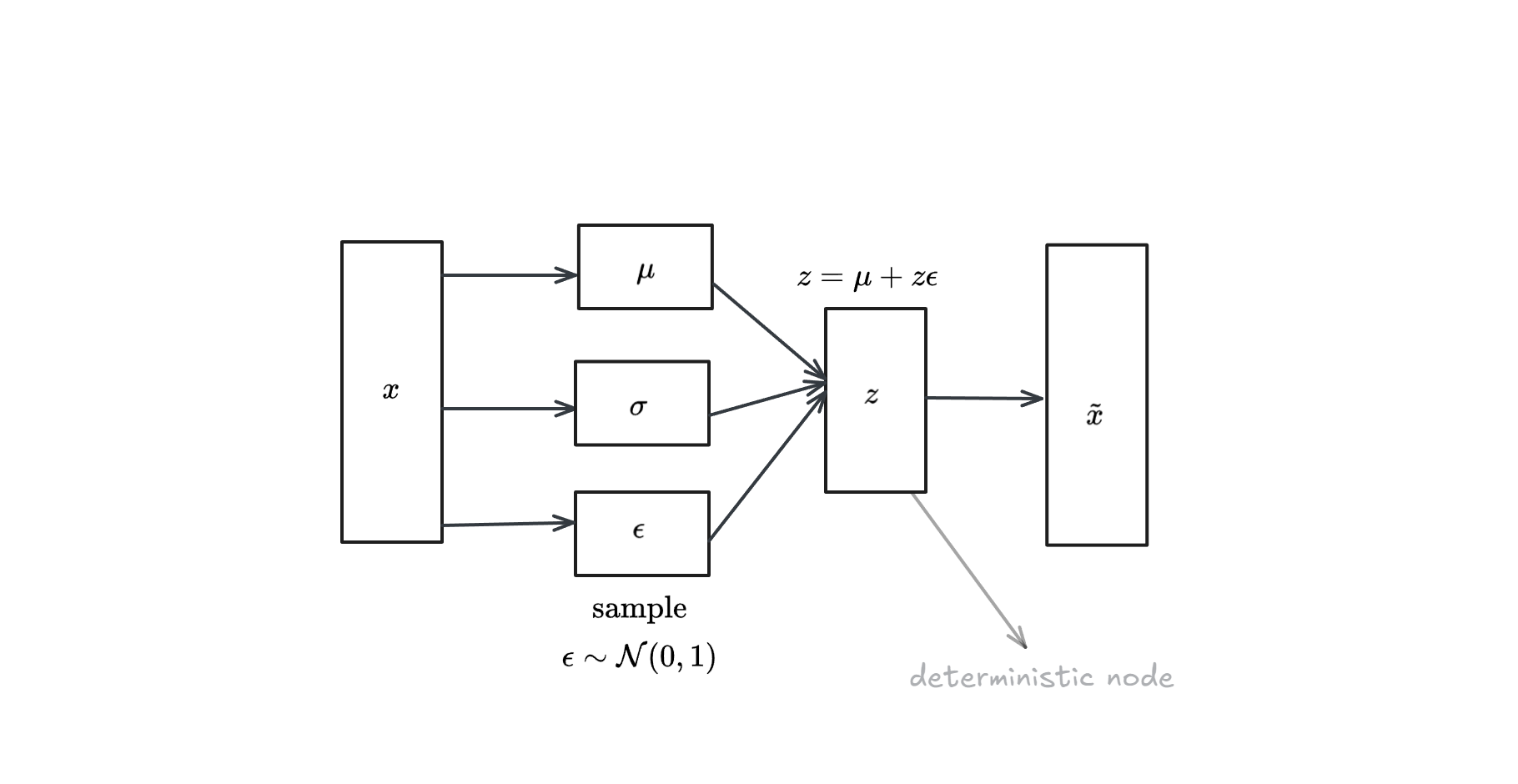
The problem we face is that we introduce a probabilistic node, hence doing backprobagation to this node is not possible. To remove this node, we can use the reparametrization trick:
Generative Adversarial Network (GAN)
It’s a generator-descriminator network.
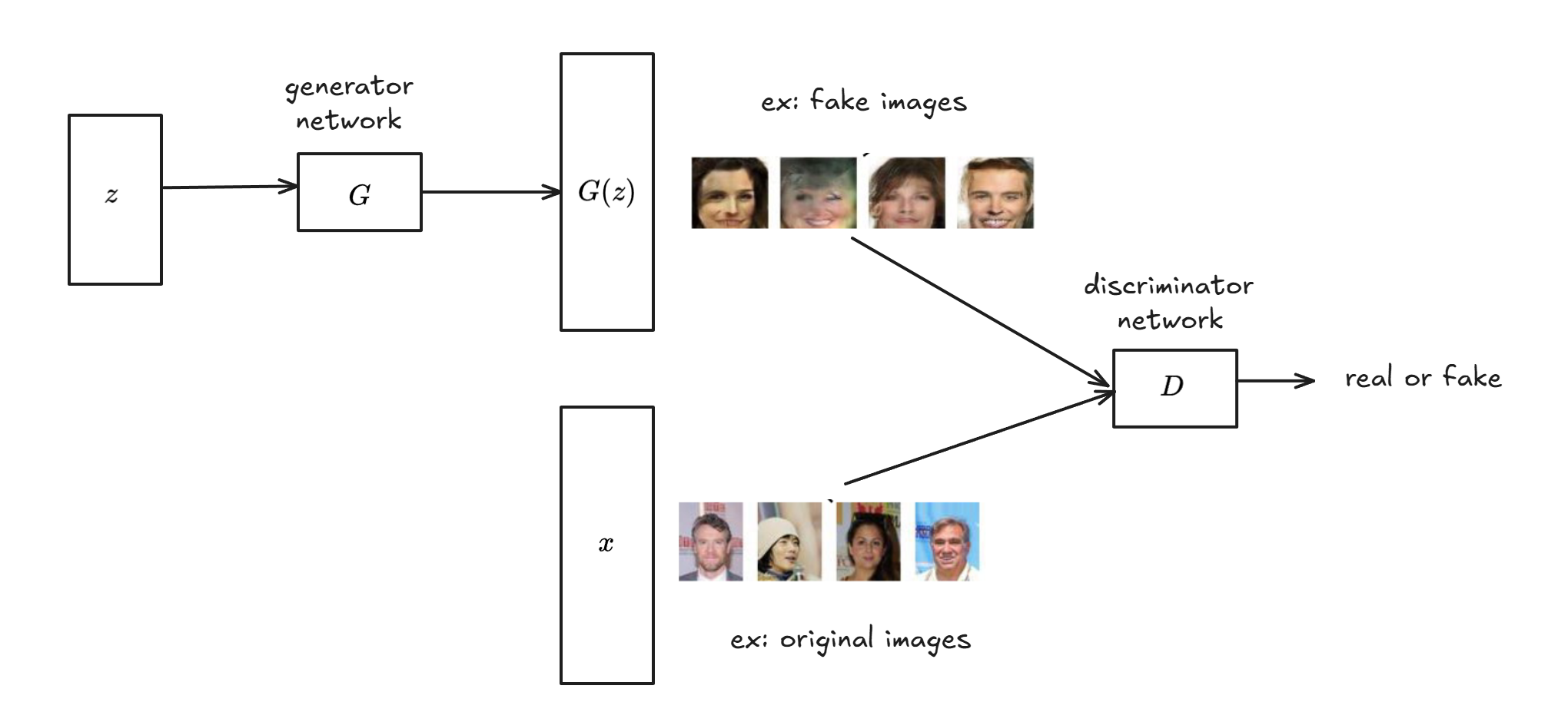
The output of this network is either
- $D(G(z))$
- $D(x)$
Ideally we want:
$$C = min_G max_D \mathbb{E}[log(D(x))] - \mathbb{E} [log(1-D(G(x)))]$$