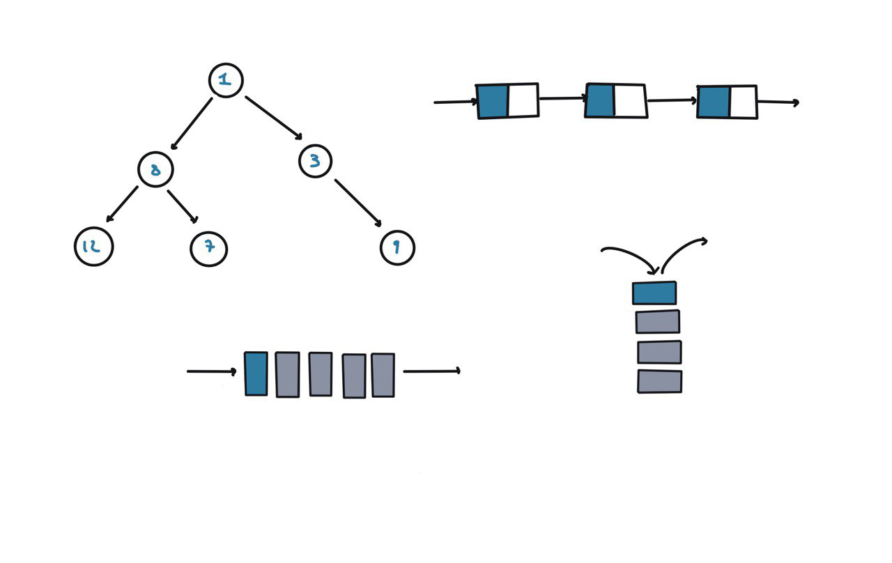
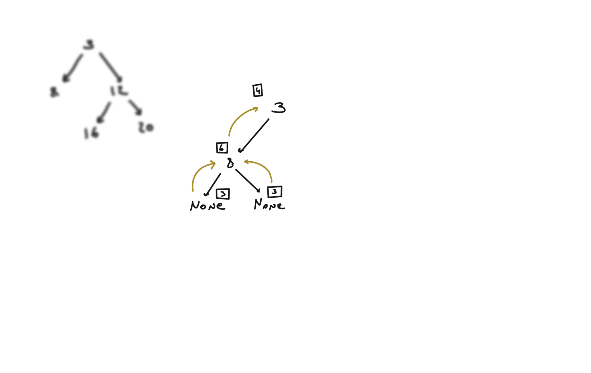
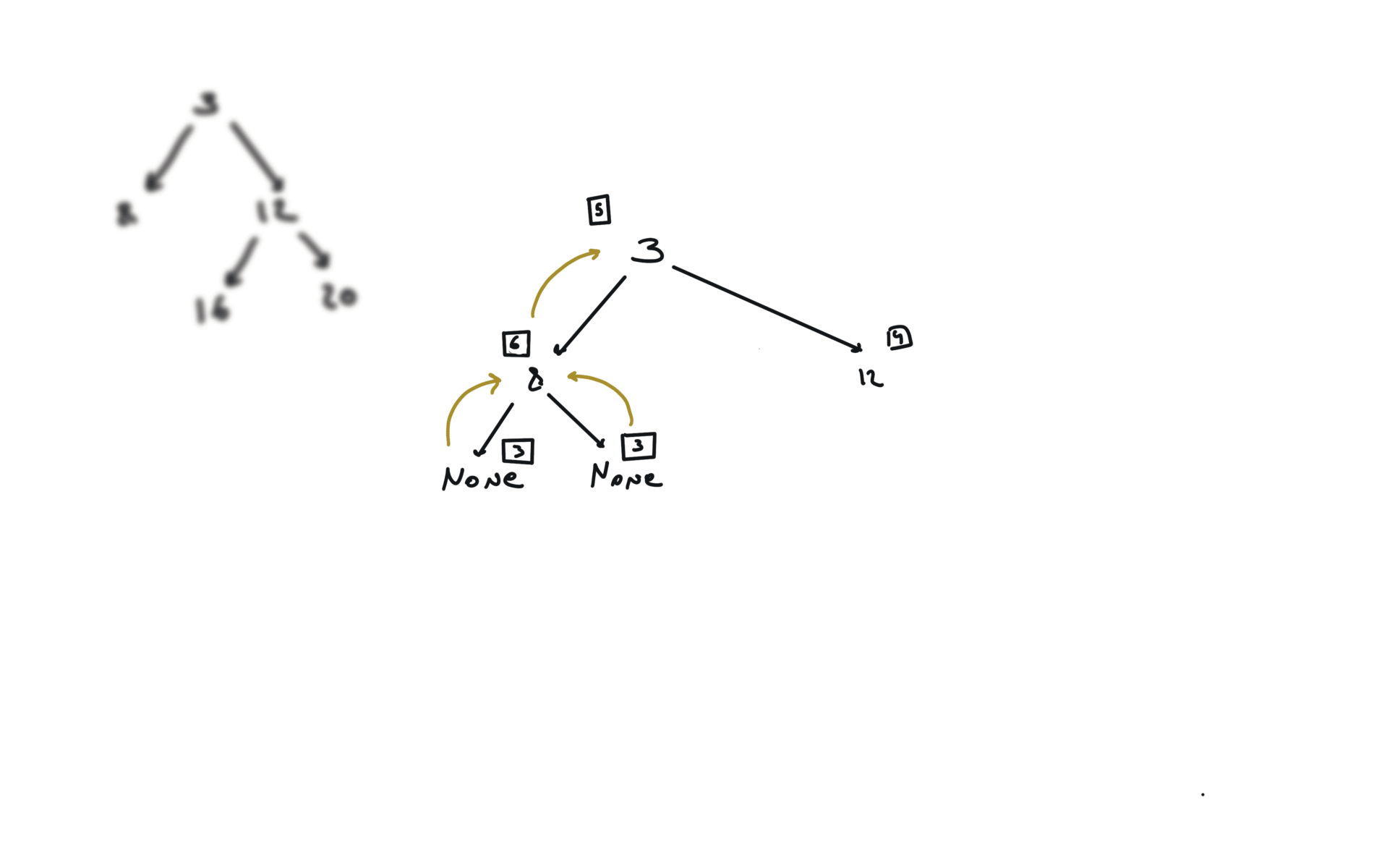
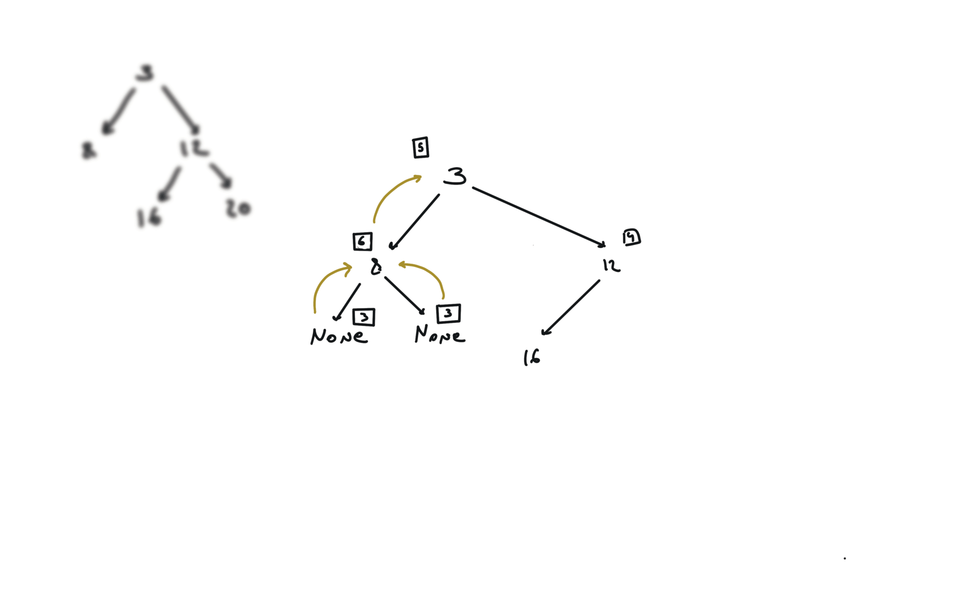
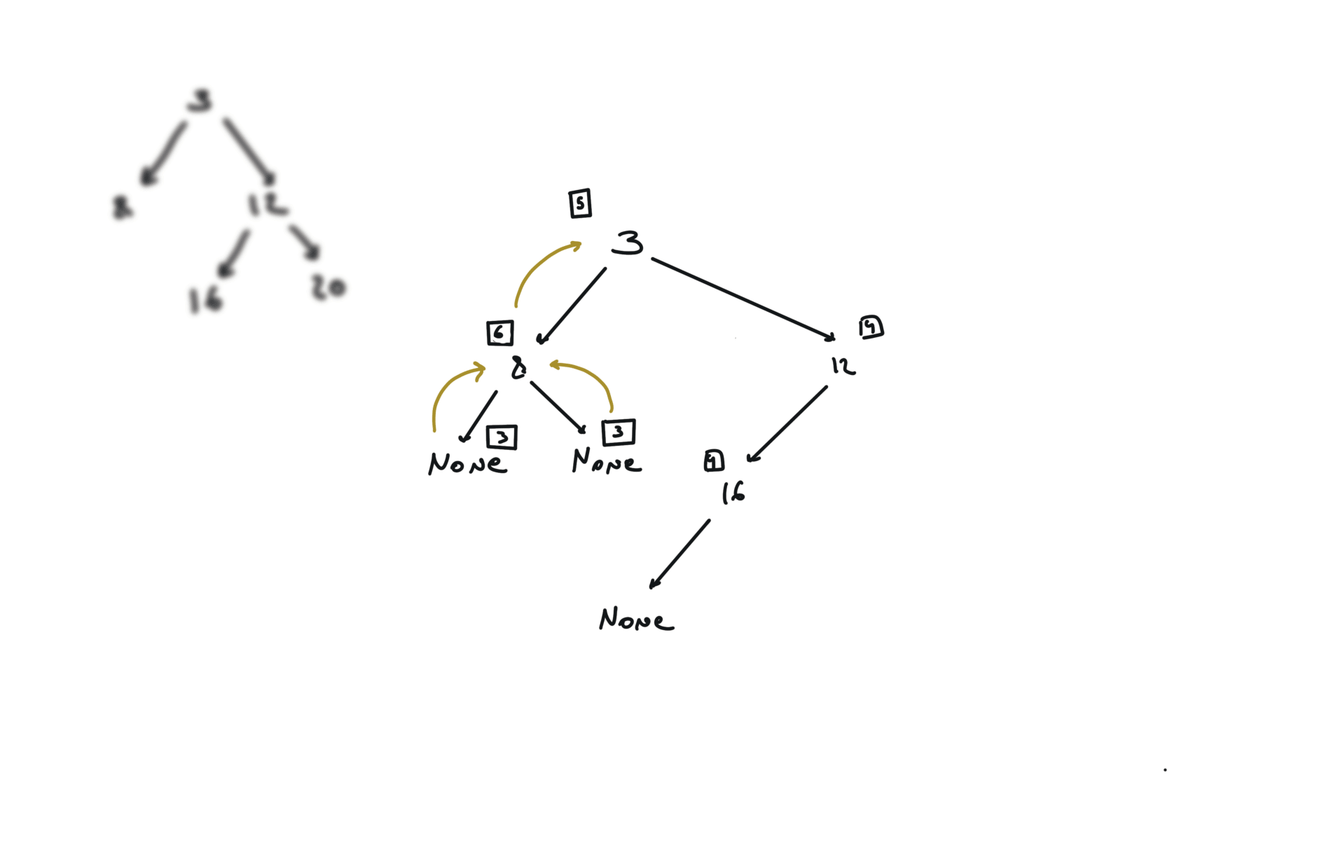
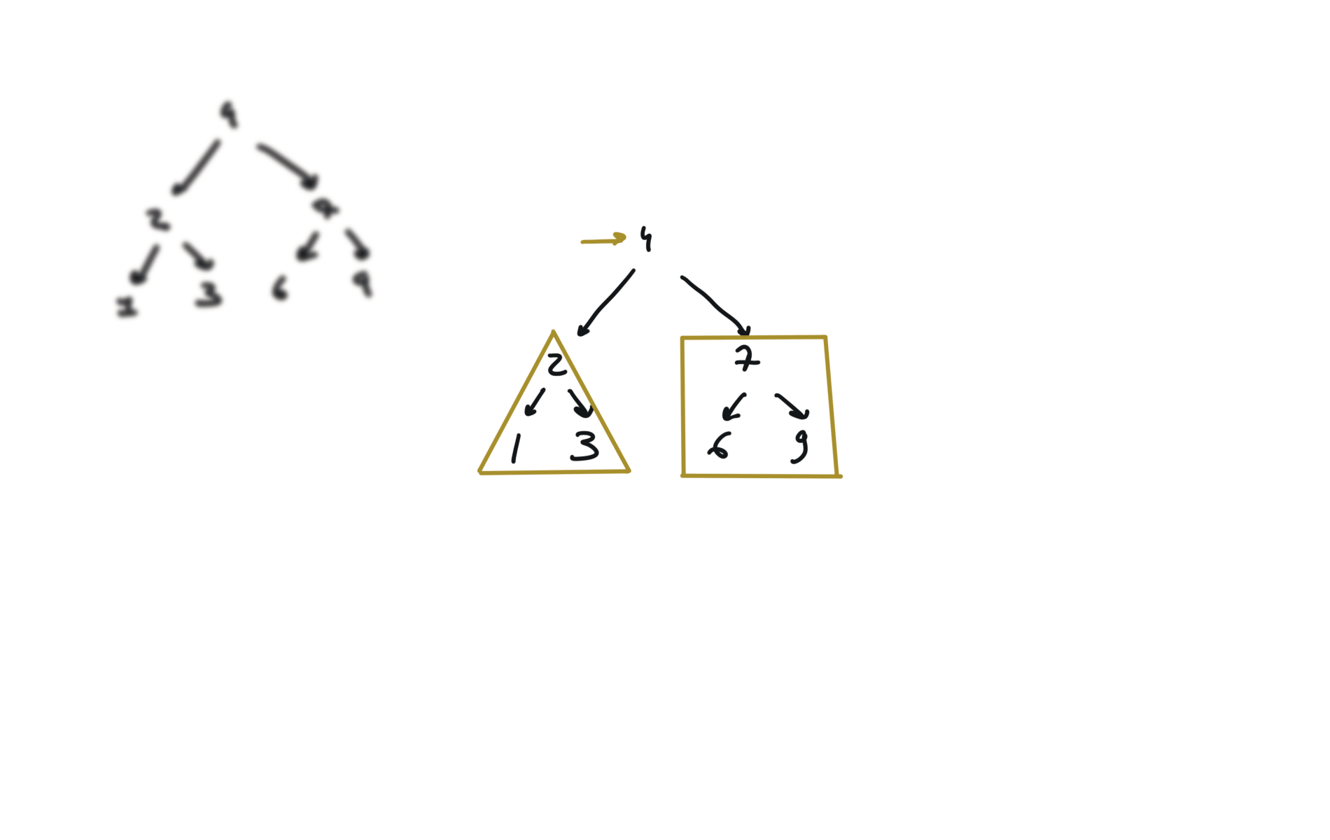
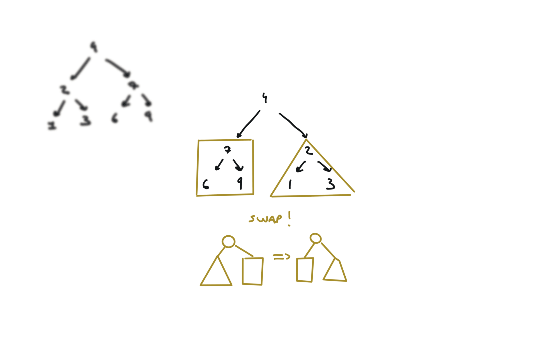
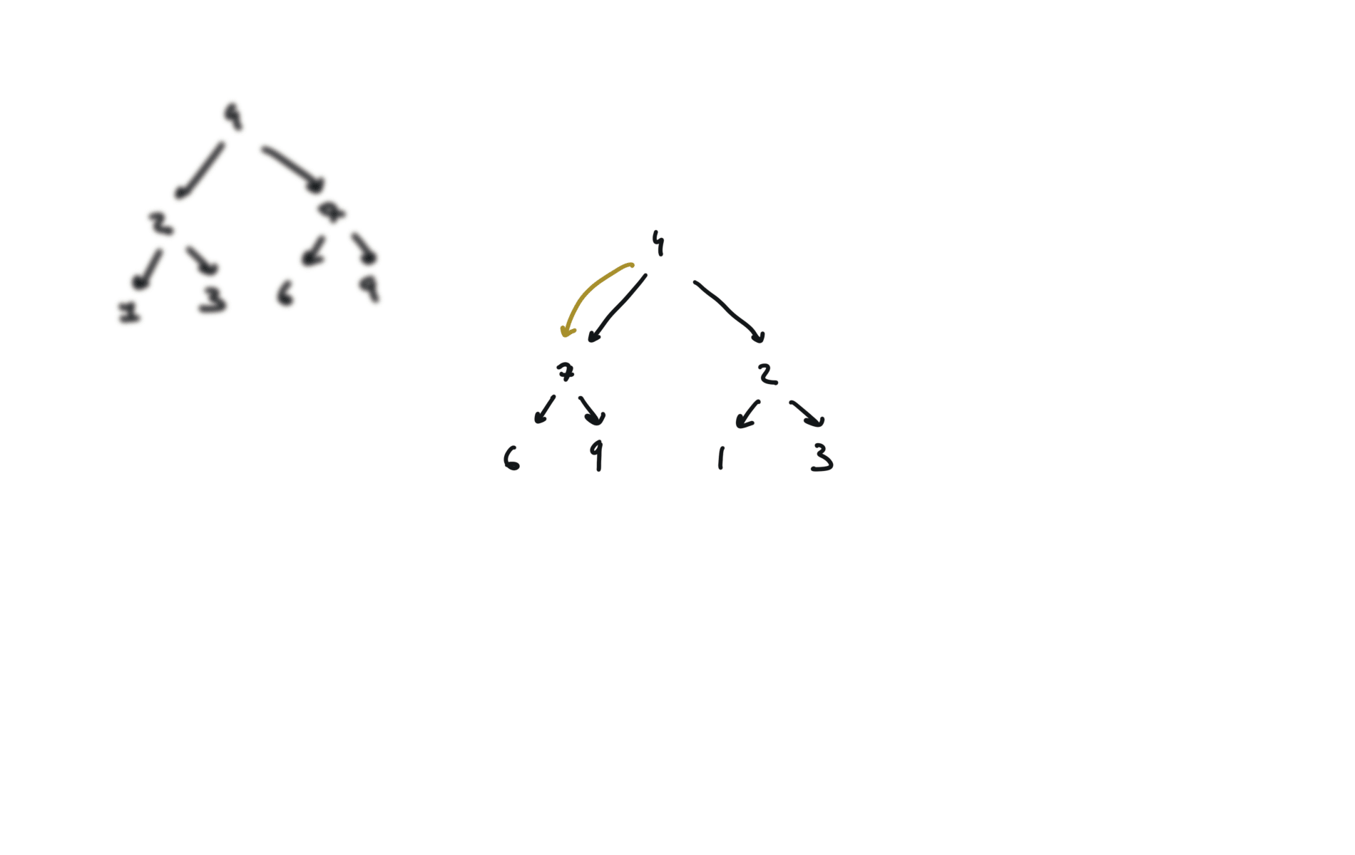
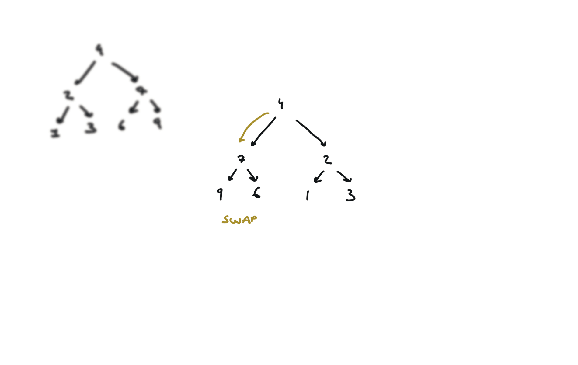
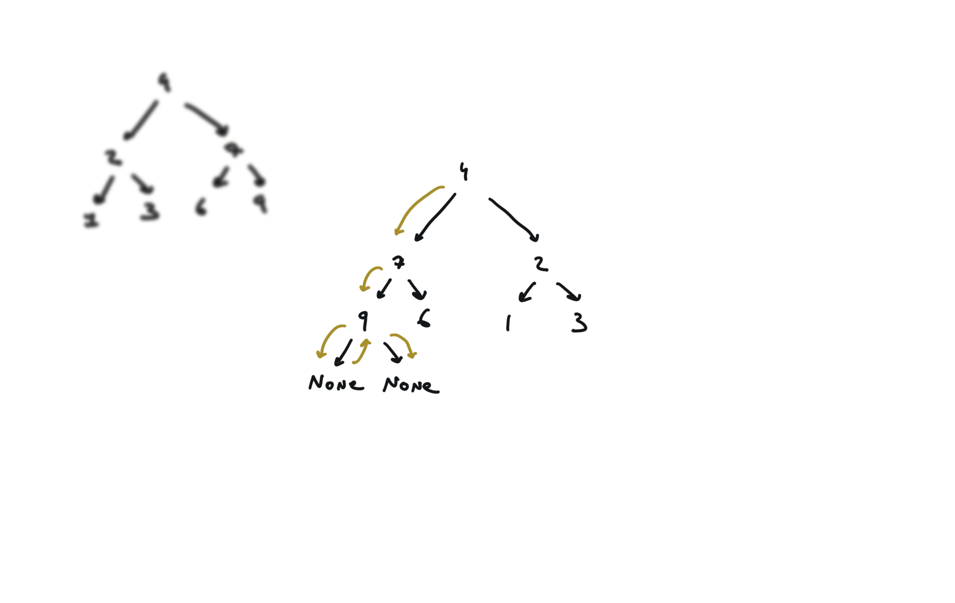
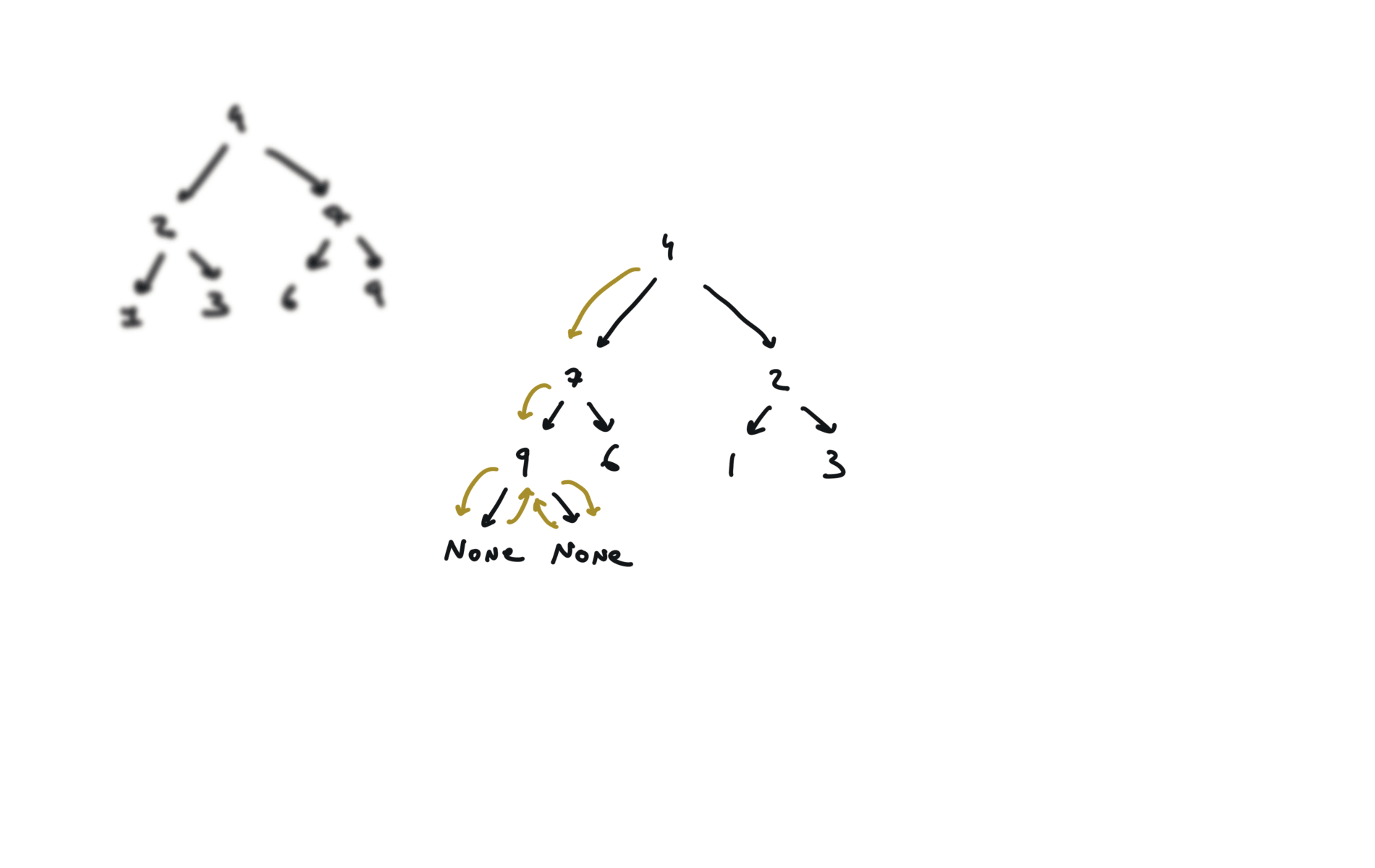
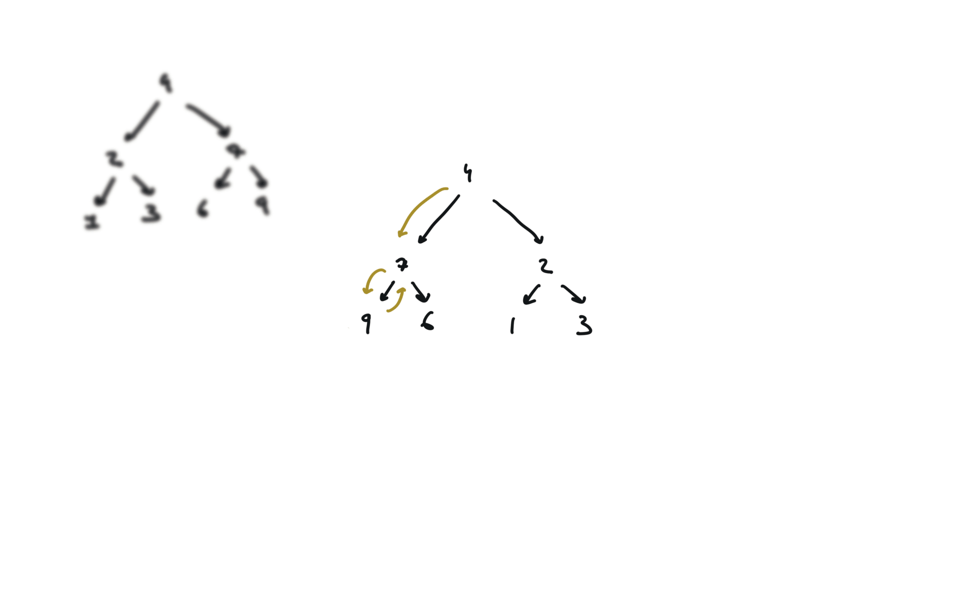
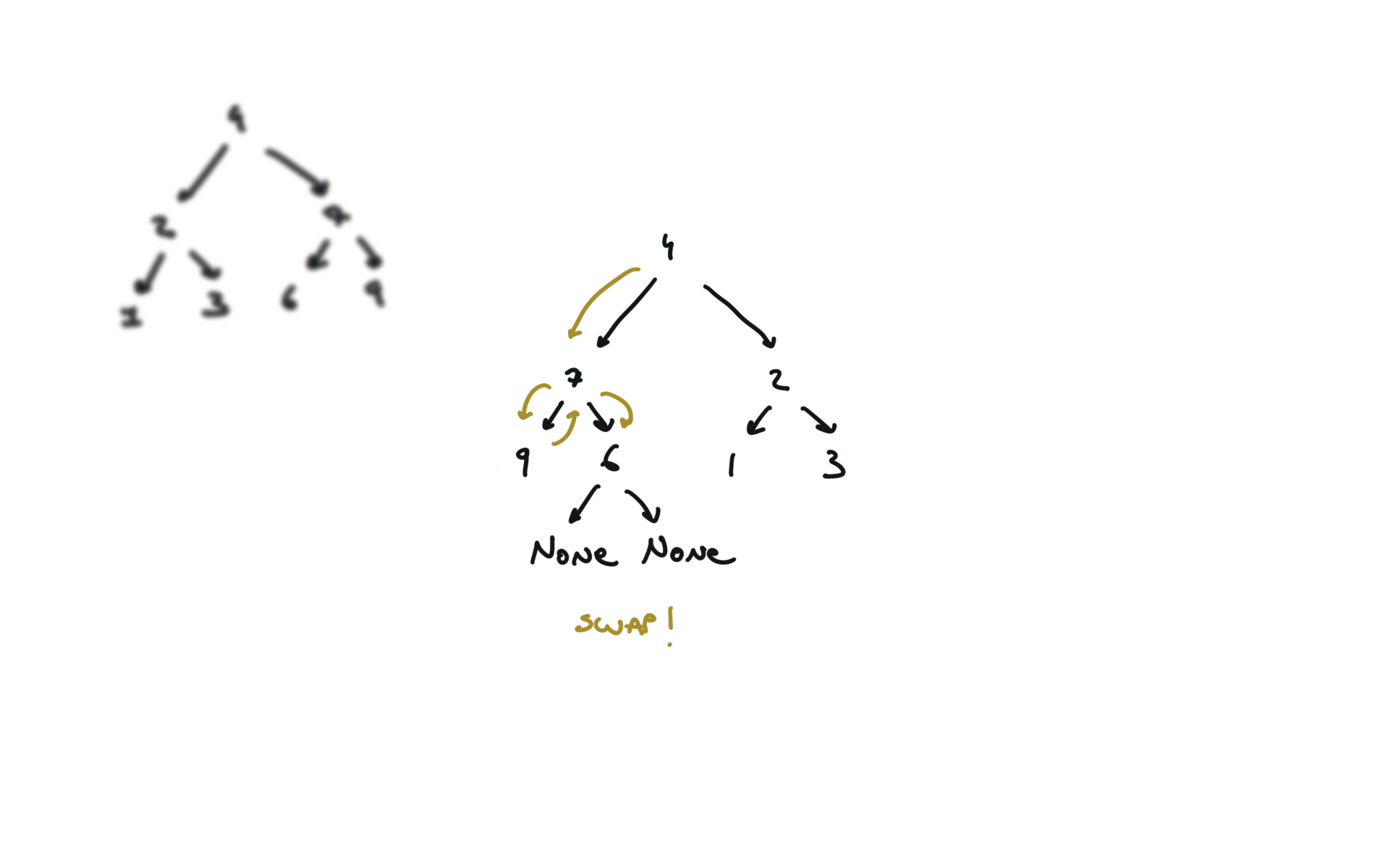
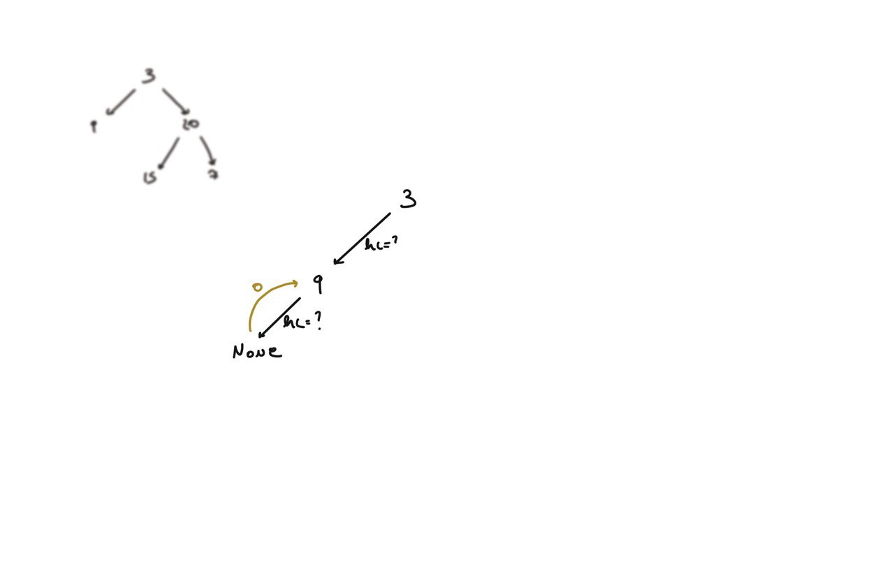
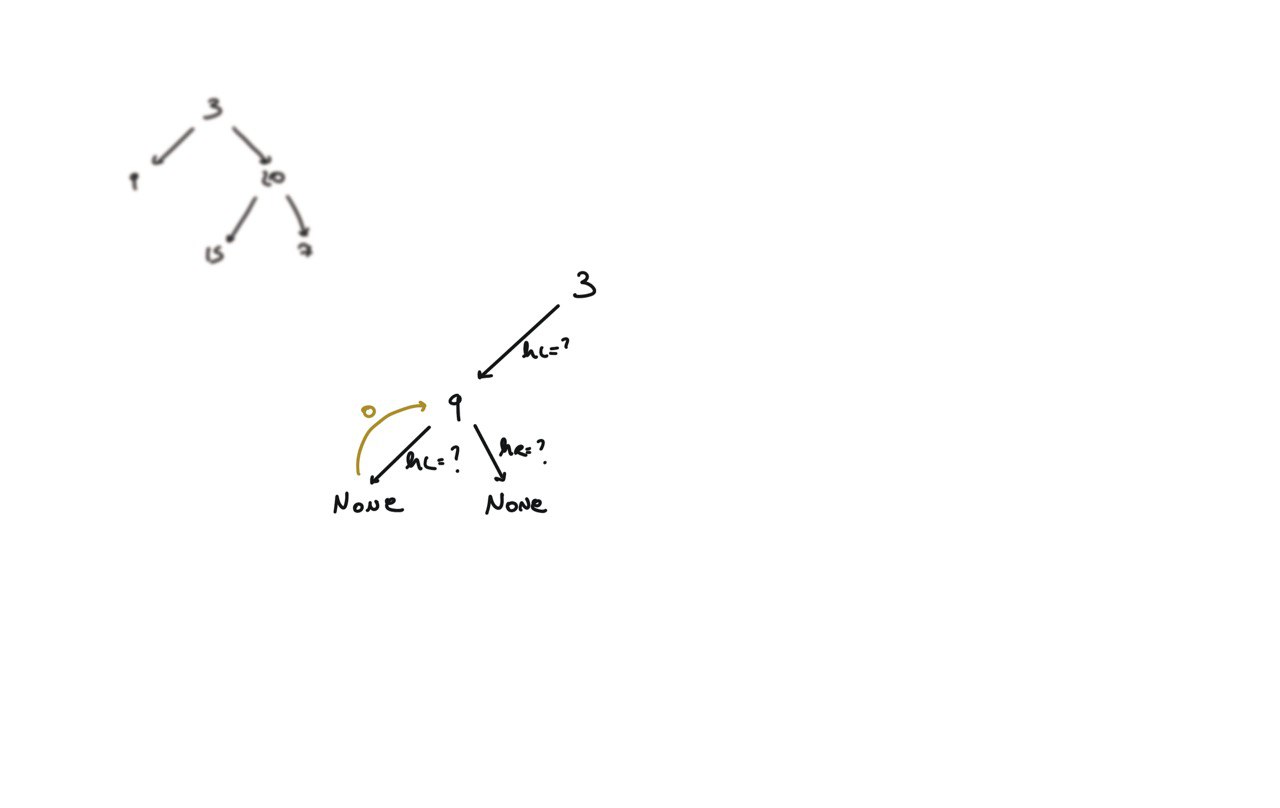
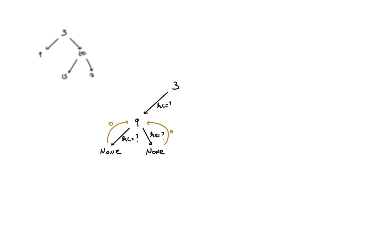
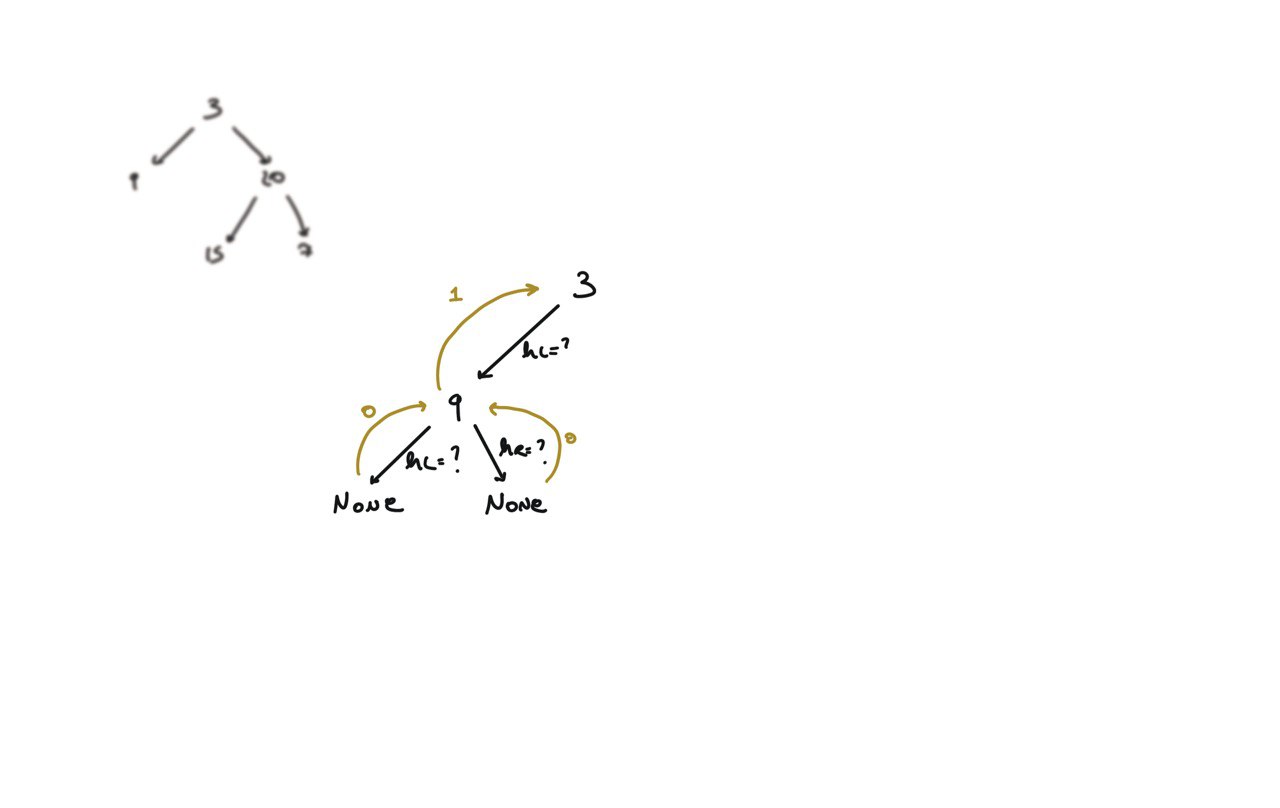
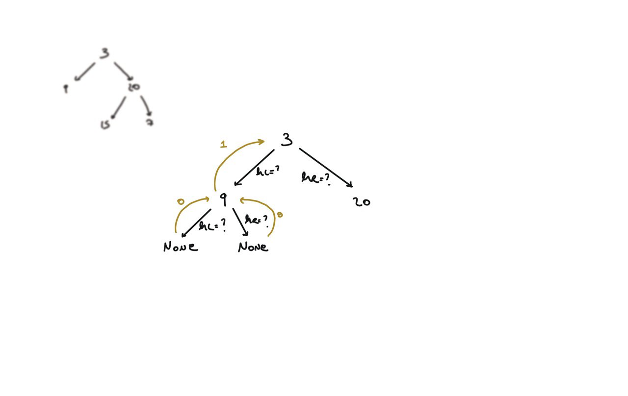
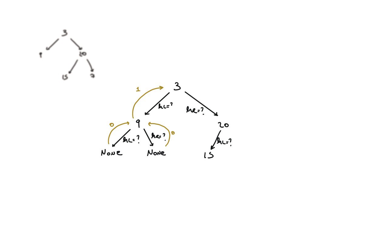
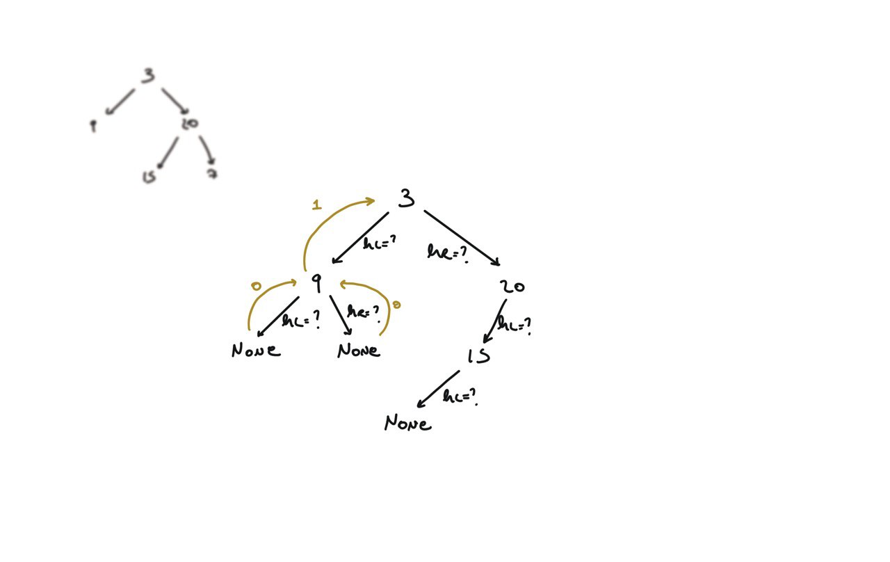
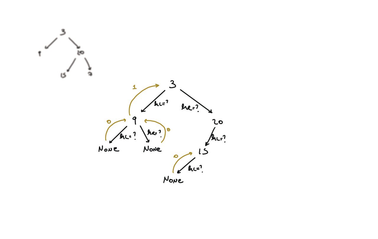
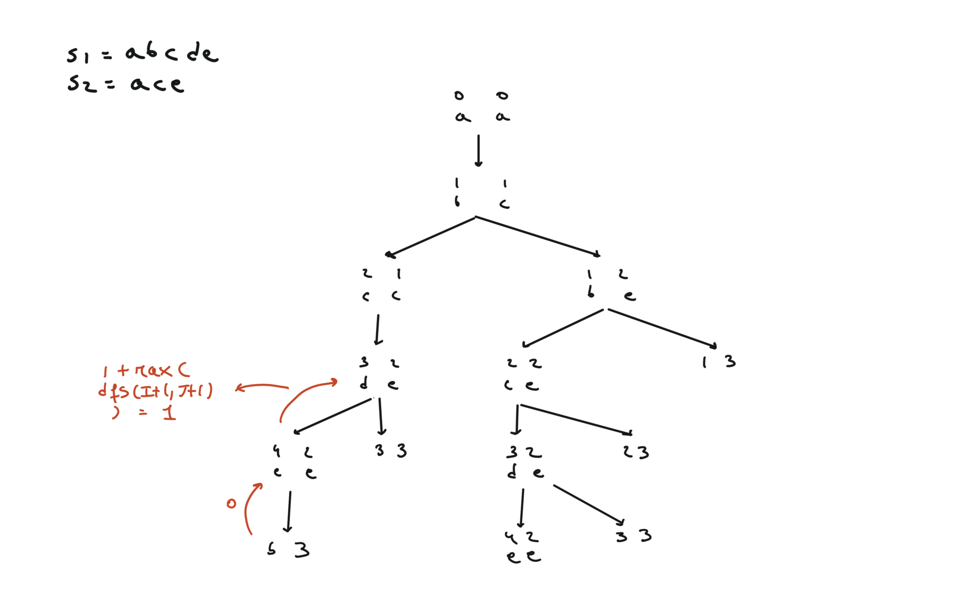
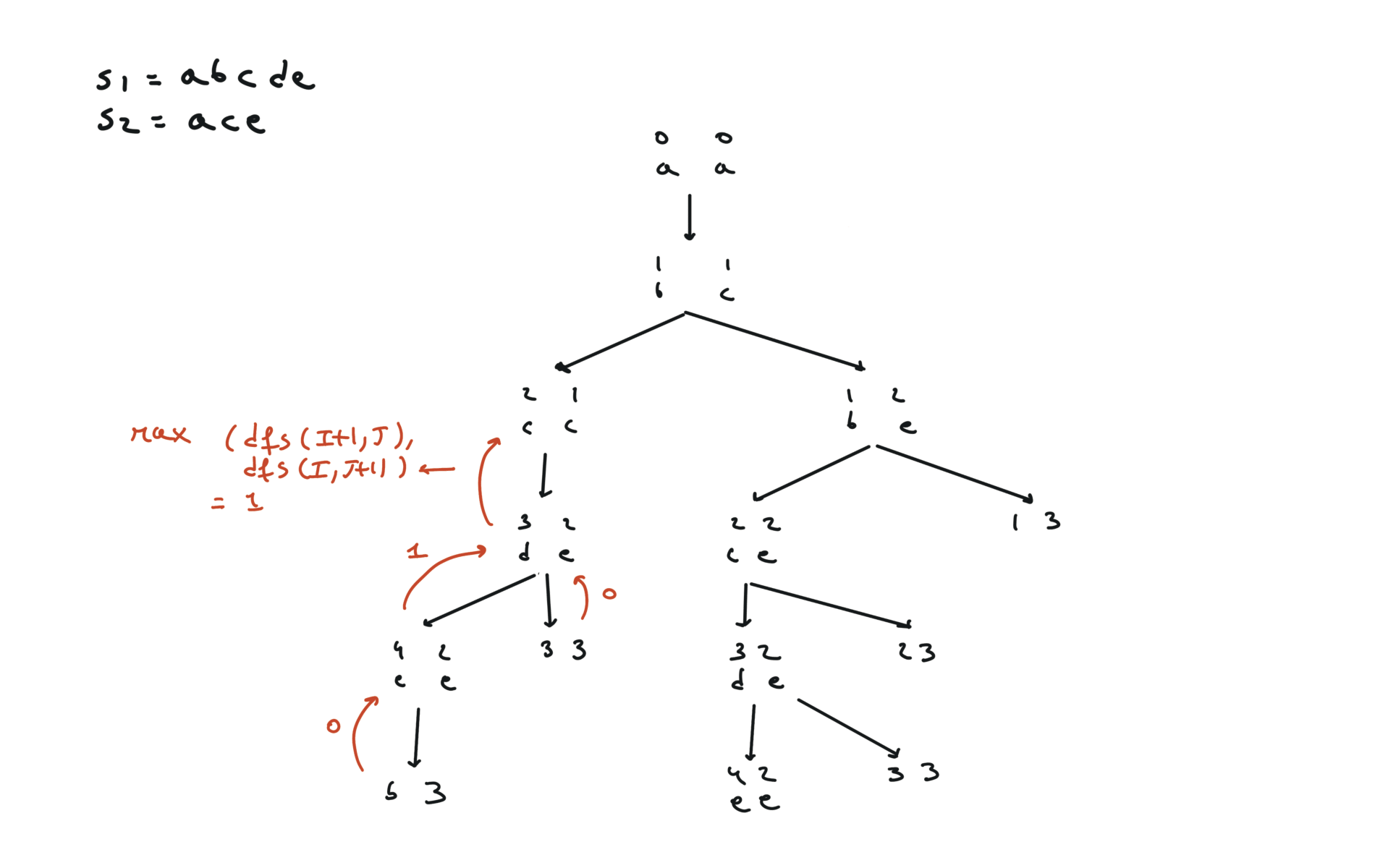
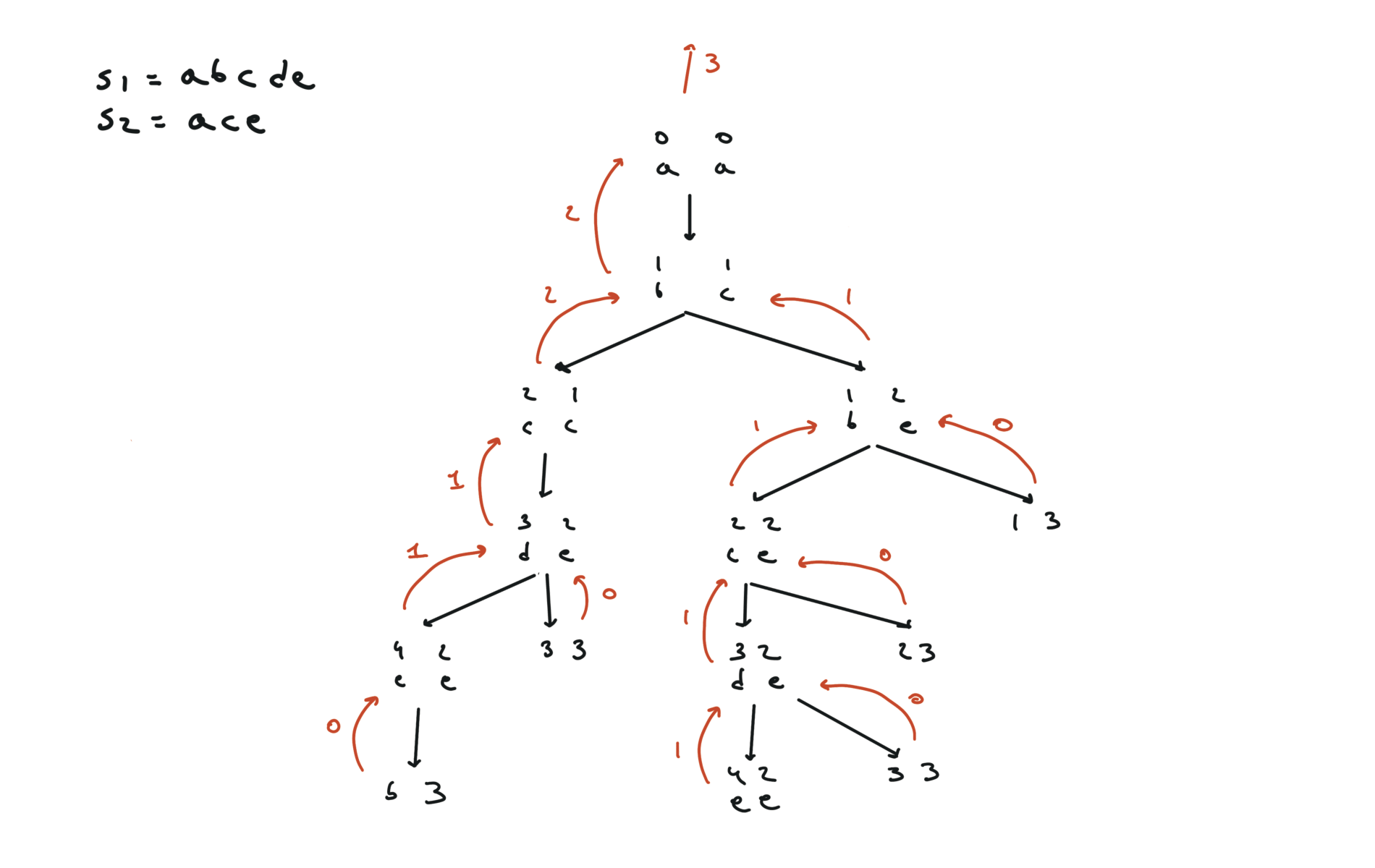
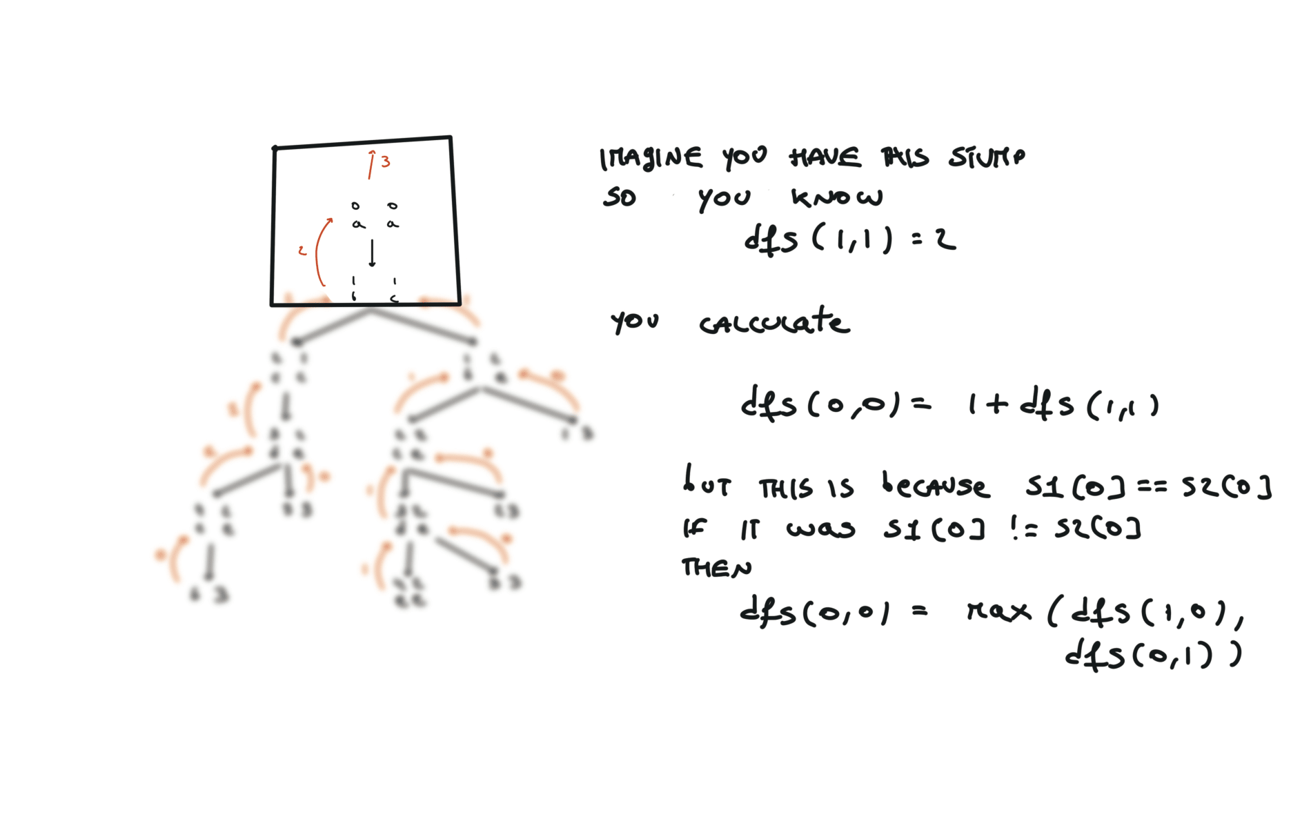
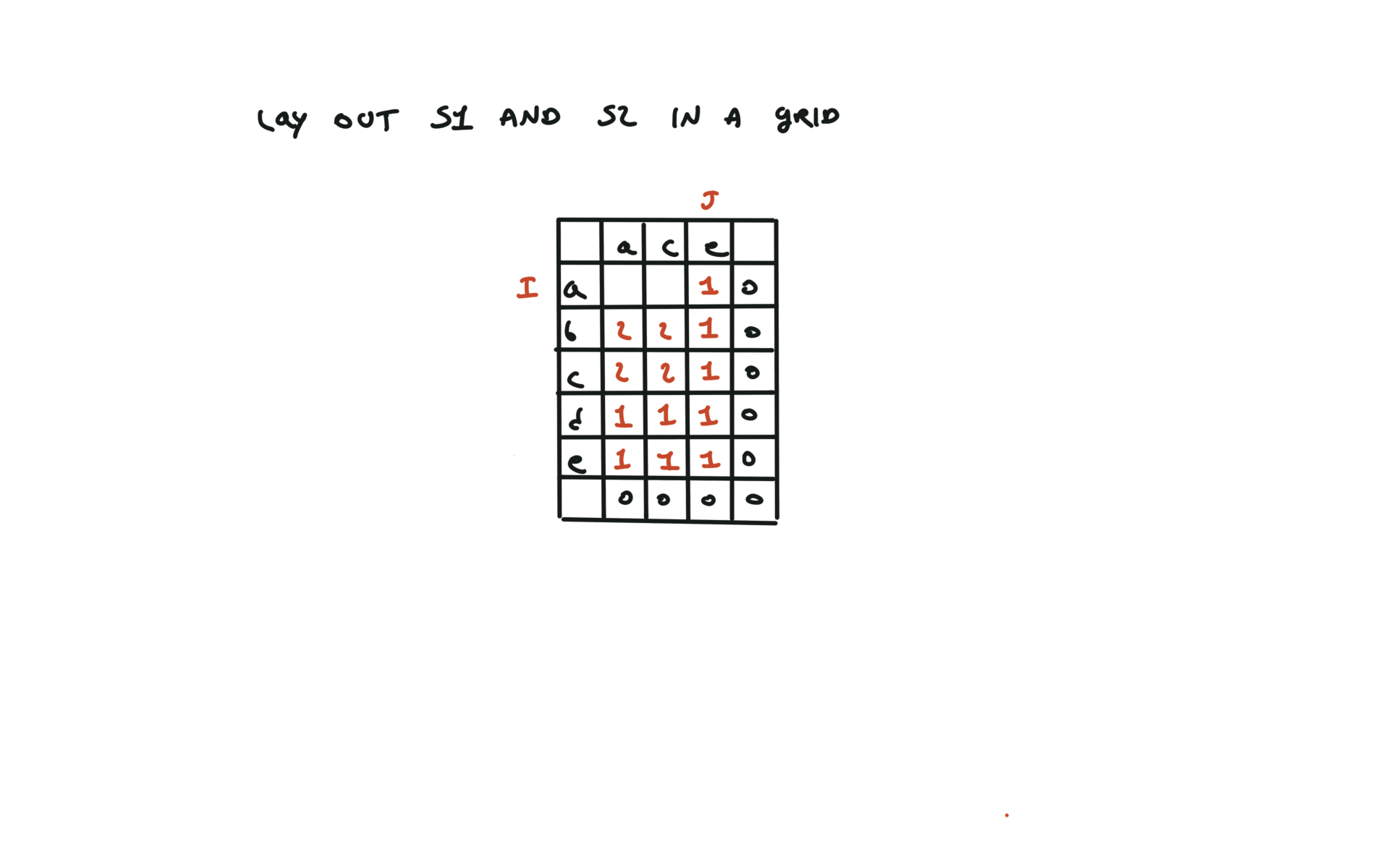
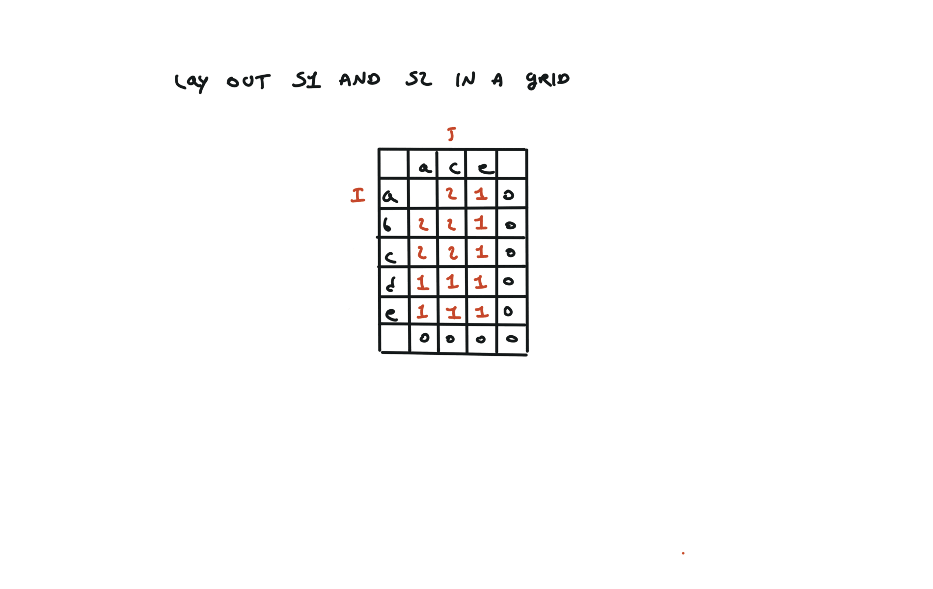
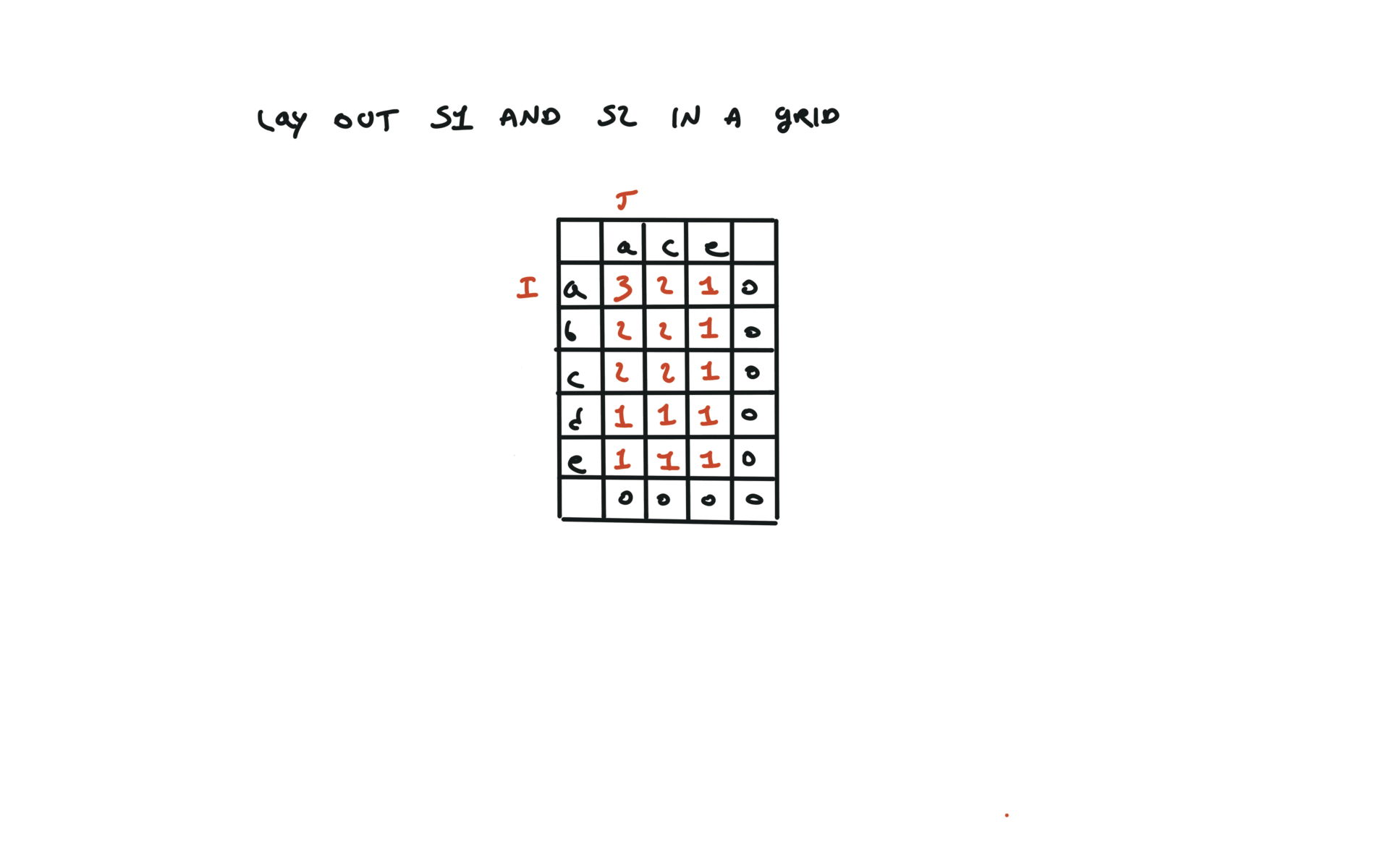
This project is primarily for me. It’s a way to organize my leetcode solutions in a way that’s easily searchable and comparable. Also because I’ve noticed that many resources, especially when it comes to dynamic programming problems, often skip over the naive or memoized solutions, jumping straight to the optimized versions. I believe understanding these intermediate steps is crucial, so I aim to include them wherever relevant.
My goals with this blog are:
- To create a more intuitive categorization of problems, making it easier to find and revisit specific types of challenges.
- To provide visualizations that help explain the solutions, along with code that directly reflects these visualizations.
Not all solutions have visual aids just yet, but they will be added over time as I continue to build and refine this space.
Sorting
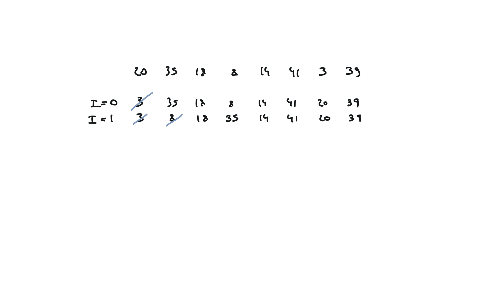
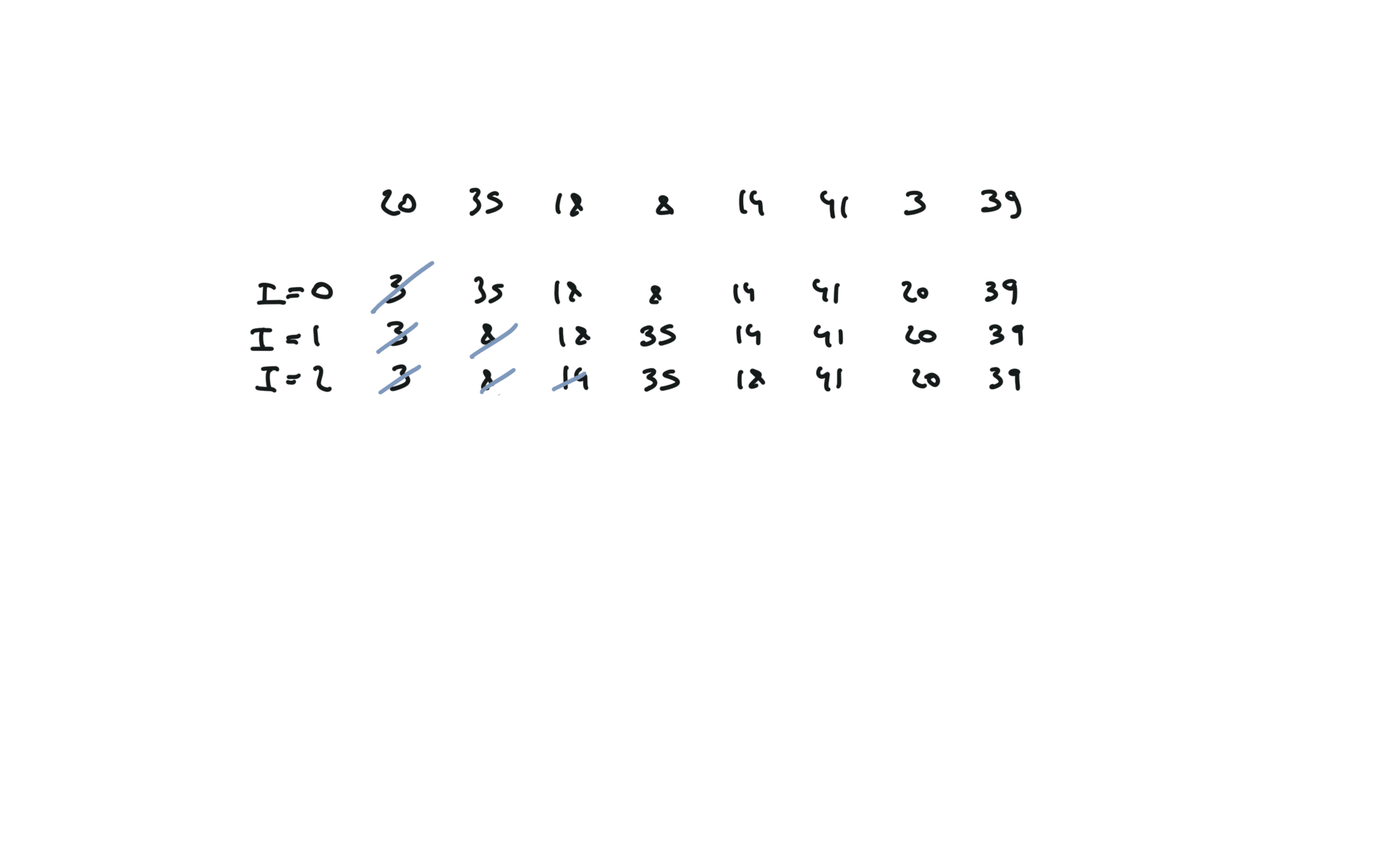
Because for $i=0$ we have $n-1$ comparisons, for $i=1$ we have $n-2$ comparisons, …, for $i=n-2$ we have $1$ comparison.
The number of comparisons is then $ \sum_{i=0}^{n-1} i = \frac{n(n-1)}{2}$ Selection sort is NOT stable. Insertion sort IS stable.
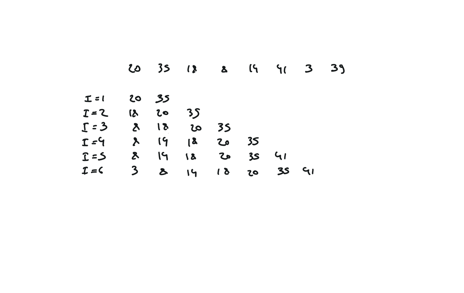
Because for $i=n-1$ we have $n-1$ comparisons, for $i=n-2$ we have $n-2$ comparisons, …, for $i=1$ we have $1$ comparison.
The number of comparisons is then $ \sum_{i=0}^{n-1} i = \frac{n(n-1)}{2}$
Bubble sort IS stable. Slightly better algorithm with flag: You can use any stable algorithm to sort each bucket. Heapify complexity is $O(n)$, heappop complexity is $O(log_2n)$, hence:
$$T(n) = O(nlog_2n)$$
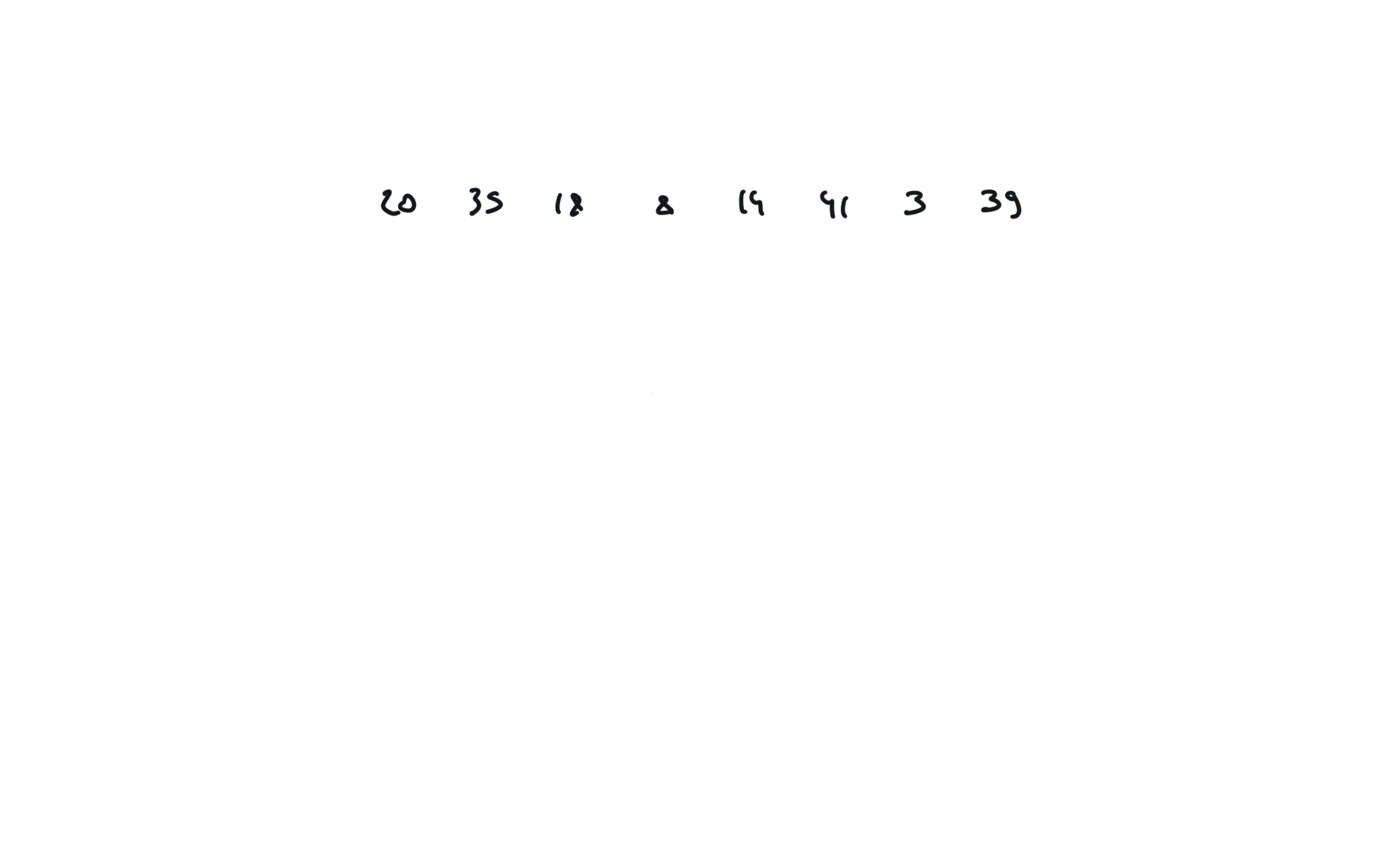
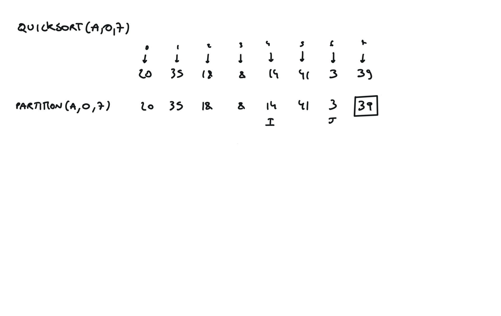
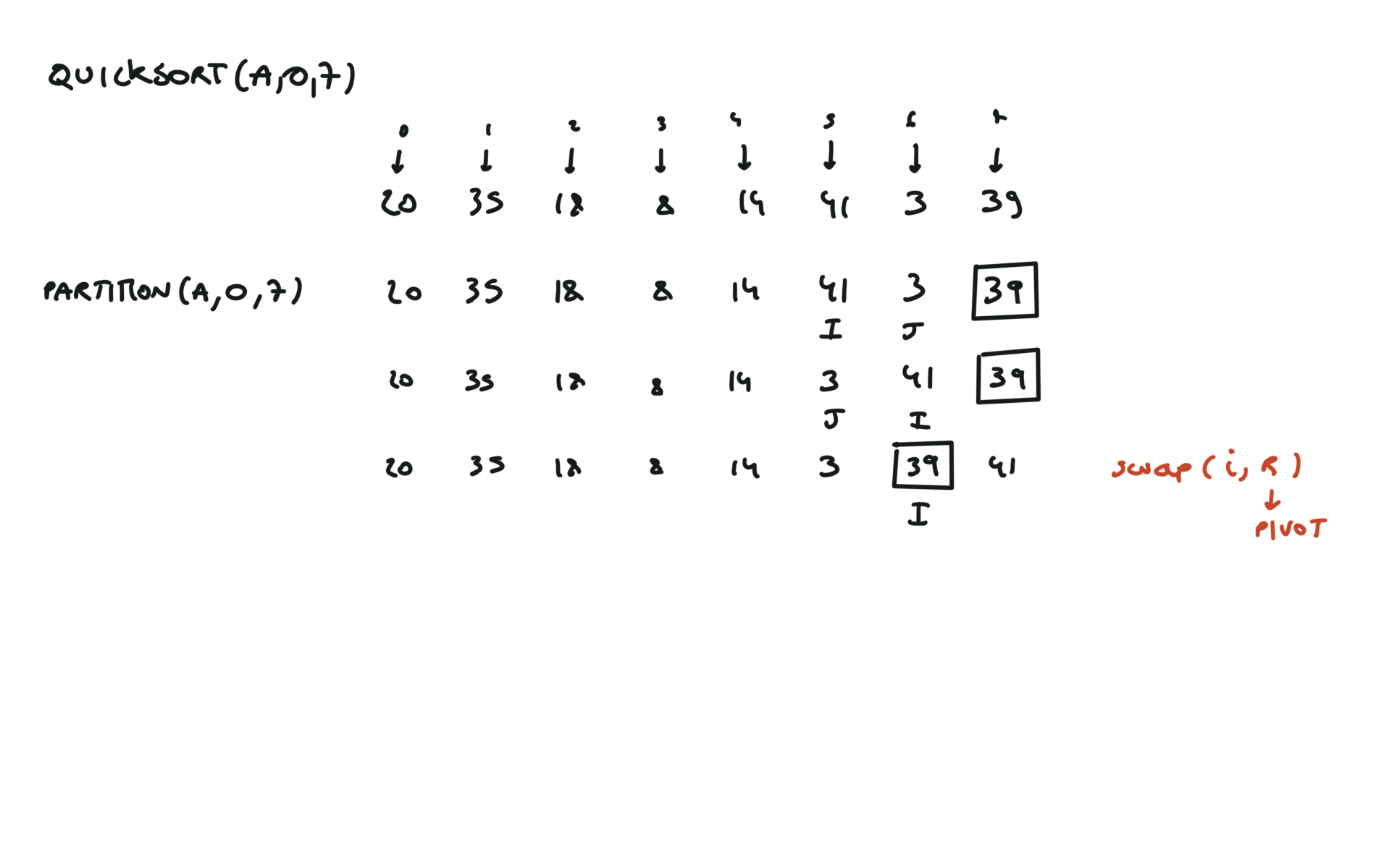
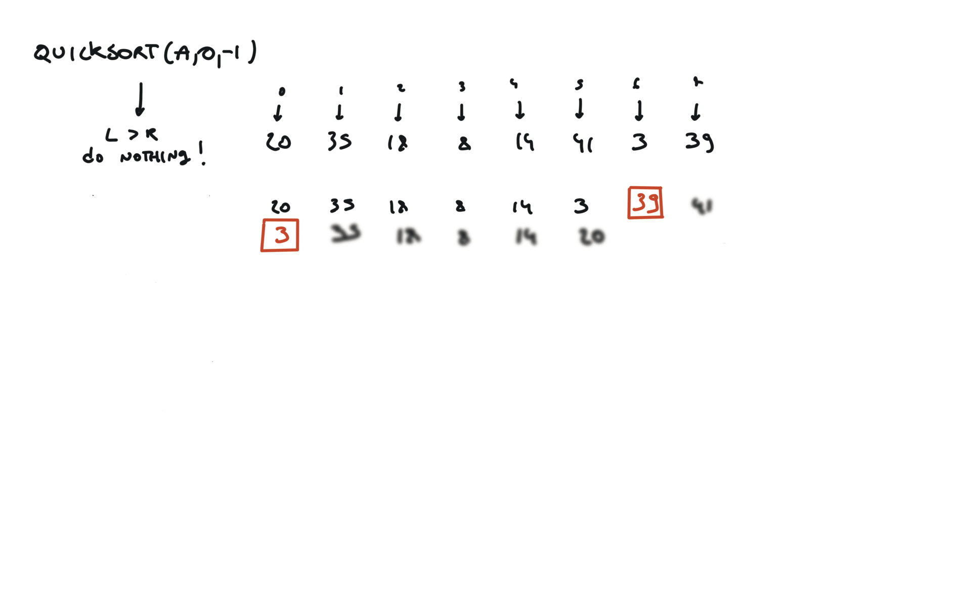
Heap sort is NOT stable On the best case scenario, every partition divide the array in half
$$T(n) = 2T(\frac{n}{2}) + n$$
$$\rightarrow T(n) = O(nlog_2n)$$ On the worst case scenario, the array is already sorted
$$T(n) = T(n-1) + n$$
$$\rightarrow T(n) = O(n^2)$$ On the average case scenario, the array is already sorted
$$T(n) = \frac{1}{n} \sum_{k=1}^{n} (T(k-1) + T(n-k-1)) + n$$
$$\rightarrow T(n) = O(nlog_2n)$$ Because we have to sum every case a[0]|—k—| P |—(n-k-1)—|a[n-1] and get the average.
Quick sort is NOT stable.
$$T(n) = 2T(\frac{n}{2}) + n$$
$$\rightarrow T(n) = O(nlog_2n)$$
Merge sort IS stable. You can also use The catch with sorted is that it can be used to sort tuples while If the array is made of tuple it will always sort by the first element of the tuple: You can specify how to sort the array with the key parameter.
E.g you want the array to be sorted in reverse: Same thing for the sorted method. key parameter can also be used to specify how to order in case we have a matching in the first tuple element: In this case we have a matching in the tuple (9,77), (9,99) and it is sorted decreasingly for the second element of the tuple. You can also solve this problem with heap, the solution with heap will have a complexity of $O(nlogk)$ while this solution is $O(n)$.sorting
selection sort
def selection_sort(a):
    for i in range(0,len(a) - 1):
        minn = i
        for j in range(i+1, len(a)):
            if a[j] < a[minn]:
                minn = j
        a[minn], a[i] = a[i], a[minn]
visualization
time complexity
insertion sort
def insertion_sort(a):
    for i in range(1, len(a)):
        v = a[i]
        j = i
        while j > 0 and a[j - 1] > v:
            a[j] = a[j - 1]
            j -= 1
        a[j] = v
visualization
bubble sort
def bubble_sort(a):
    for i in range(len(a)-1, 0, -1):
        for j in range(1, i + 1):
            if a[j - 1] > a[j]:
                a[j - 1], a[j] = a[j], a[j - 1]
visualization
time complexity
def bubble_sort_flag(a):
    i = len(a) - 1
    sorted = False
    while i >= 1 and not sorted:
        sorted = True
        for j in range(1,i + 1):
            if a[j - 1] > a[j]:
                a[j - 1], a[j] = a[j], a[j - 1]
                sorted = False
        i = i - 1
bucket sort
def bucket_sort(arr):
    n = len(arr)
    buckets = [[] for _ in range(n)]
    for num in arr:
        bi = int(n * num)
        buckets[bi].append(num)
    for bucket in buckets:
        insertion_sort(bucket)
    index = 0
    for bucket in buckets:
        for num in bucket:
            arr[index] = num
            index += 1
arr = [0.78, 0.17, 0.39, 0.26, 0.72, 0.94, 0.21, 0.12, 0.23, 0.68]
time complexity
heap sort
import heapq

def heap_sort(arr):
    heapq.heapify(arr)
    result = []
    while arr:
        result.append(heapq.heappop(arr))
    return result
time complexity
quick sort
def partition(a, l, r):
    pivot = a[r]
    i, j  = l, r - 1
    while True:
        while a[i] < pivot:
            i += 1
        while a[j] > pivot and j > 0:
            j -= 1
        if i >= j:
            break
        a[i], a[j] = a[j], a[i]
    a[i], a[r] = a[r], a[i]
    return i

def quicksort(a, l, r):
    if l < r:
        pi = partition(a, l, r)
        quicksort(a, l, pi - 1)
        quicksort(a, pi + 1, r)
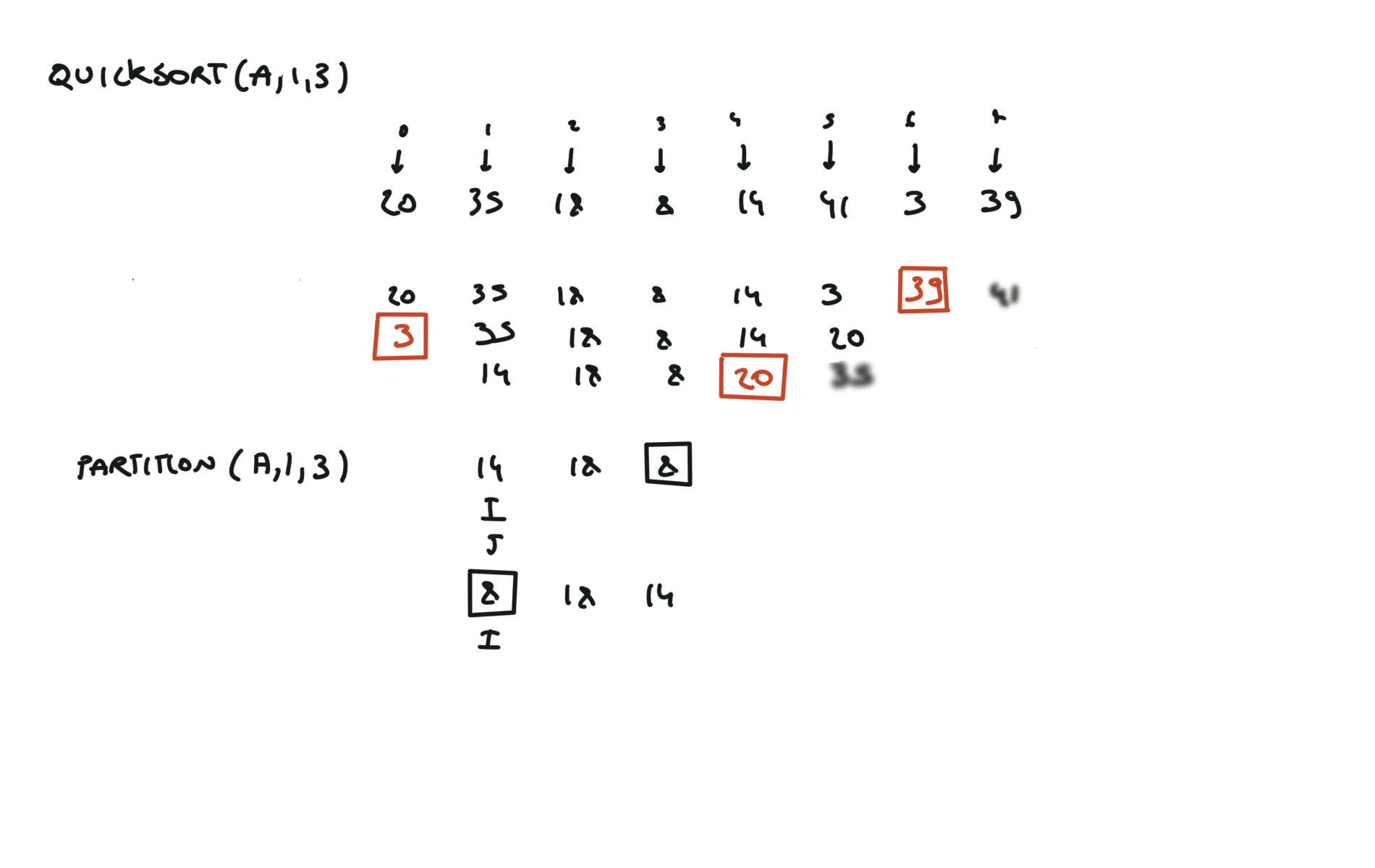
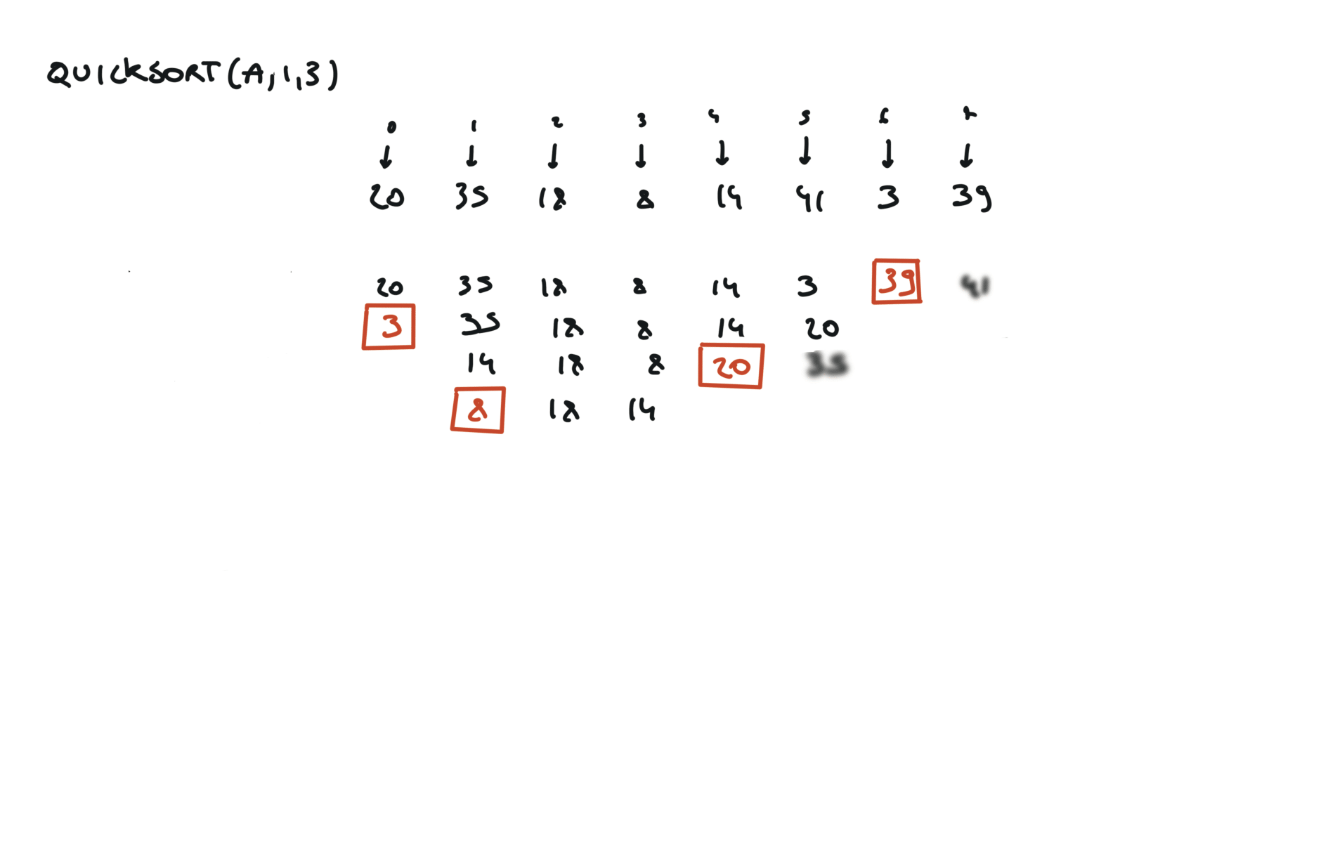
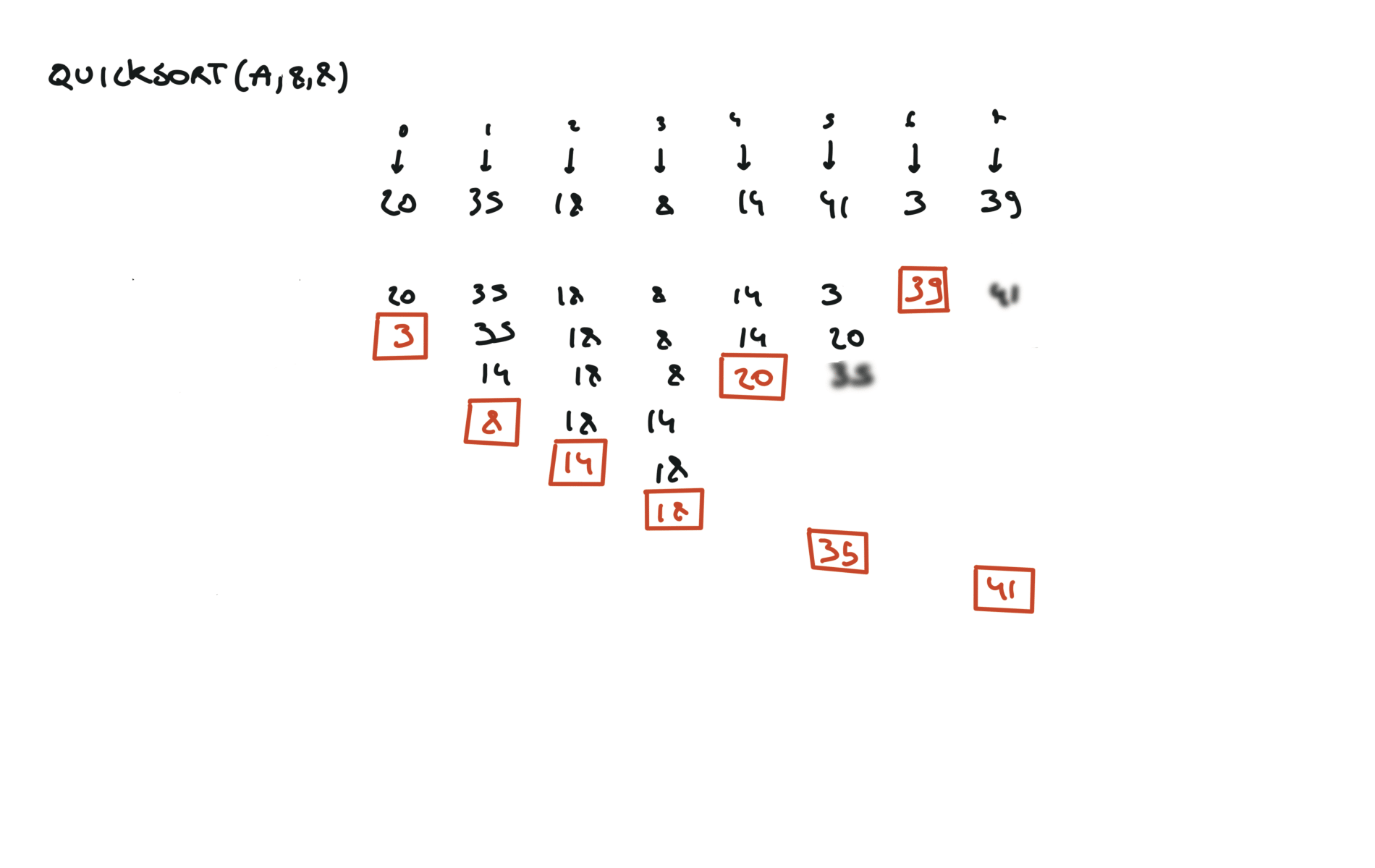
visualization
time complexity
merge sort
def merge(a, l, m, r):
    n1 = m - l + 1
    n2 = r - m
    L = [0] * n1
    R = [0] * n2
    for i in range(n1):
        L[i] = a[l + i]
    for j in range(n2):
        R[j] = a[m + 1 + j]

    i, j, k = 0, 0, l
    while i < n1 and j < n2:
        if L[i] <= R[j]:
            a[k] = L[i]
            i += 1
        else:
            a[k] = R[j]
            j += 1
        k += 1

    while i < n1:
        a[k] = L[i]
        i += 1
        k += 1
    while j < n2:
        a[k] = R[j]
        j += 1
        k += 1

def mergesort(a, l, r):
    if l < r:
        m = (r + l) // 2
        mergesort(a, l, m)
        mergesort(a, m + 1, r)
        merge(a, l, m, r)
visualization
time complexity
sorting in python
a = [6, 9, 2, 9, 90, 18]
a.sort() # -> [2, 6, 9, 9, 18, 90]
sorted like thisa = [6, 9, 2, 9, 90, 18]
a = sorted(a) # -> [2, 6, 9, 9, 18, 90]
tuple.sort() won’t worka = (6, 9, 2, 9, 90, 18)
# a.sort() # a is not an array
a = sorted(a) # now a will be a sorted array
a = [(6, 9), (2, 100), (9, 77), (90, 99), (18, 89)]
a.sort() # -> [(2, 100), (6, 9), (9, 77), (18, 89), (90, 99)]
a = [6, 9, 2, 9, 90, 18]
a.sort(key = lambda x: -x) # same as a.sort(reverse = True)
a = [(6, 9), (2, 100), (9, 77), (9, 99), (90, 99), (18, 89)]
a.sort(key = lambda x: (x[0],- x[1])) # -> [(2, 100), (6, 9), (9, 99), (9, 77), (18, 89), (90, 99)]
1636. Sort Array by Increasing Frequency
[desc]
(link)
count = Counter(nums)
nums.sort(key=lambda x: (count[x],-x))
return nums
347. Top K Frequent Elements
[desc]
(link)
n = len(nums)
counter = Counter(nums)
buckets = [0] * (n + 1)

for num, freq in counter.items():
	if buckets[freq] == 0:
		buckets[freq] = [num]
	else:
		buckets[freq].append(num)
ret = []
for i in range(n, -1, -1):
	if buckets[i] != 0:
		ret.extend(buckets[i])
	if len(ret) == k:
		break
return ret
Heap
A heap is an array $$\forall i \in [1,n/2]$$
$$arr[i] > arr[2i]$$
$$arr[i] > arr[2i + 1]$$ holds. In python this class is implemented in the heap
arr where the following relationshipclass Heap:
@staticmethod
def heapify(arr):
"""Transform the arr to a min-heap"""
n = len(arr)
for i in range(n // 2 - 1, -1, -1):
Heap._heapify_down(arr, n, i)
@staticmethod
def heappush(arr, value):
"""Adds value to the heap while keeping the heap property"""
arr.append(value)
Heap._heapify_up(arr, len(arr) - 1)
@staticmethod
def heappop(arr):
"""Remove and returns heap smallest element"""
root = arr[0]
arr[0] = arr[-1]
arr.pop()
Heap._heapify_down(arr, len(arr), 0)
return root
@staticmethod
def _heapify_down(arr, n, i):
"""Keep the min-heap property starting from position i going down in the tree"""
while True:
smallest = i
left = 2 * i + 1
right = 2 * i + 2
if left < n and arr[left] < arr[smallest]:
smallest = left
if right < n and arr[right] < arr[smallest]:
smallest = right
if smallest != i:
arr[i], arr[smallest] = arr[smallest], arr[i]
i = smallest
else:
break
@staticmethod
def _heapify_up(arr, i):
"""Keep the min-heap property starting from position i going up in the tree"""
while i != 0 and arr[(i - 1) // 2] > arr[i]:
parent = i // 2
arr[i], arr[parent] = arr[parent], arr[i]
i = parent
heapq library.
method
time complexity
heapq.heapify(arr)
$O(n)$
heapq.heppush(arr, element)
$O(log_2n)$
heapq.heappop(arr)
$O(log_2n)$
1046. Last Stone Weight
[desc]
(link)
hp = []
for i in range(len(stones)):
	hp.append(-1*stones[i])
heapq.heapify(hp)

while len(hp) > 1:
	x = heapq.heappop(hp)
	y = heapq.heappop(hp)
	if x != y:
		heapq.heappush(hp,-abs(x-y))

if len(hp) == 0:
	return 0
return -1*hp[0]
General problems
53. Maximum Subarray (sum)
[desc]
(link)
kadane's algorithm
naive solution
currMax = nums[0] #not 0 because array can be all negative
for i in range(len(nums)):
    currSum = 0
    for j in range(i,len(nums)):
        currSum += nums[j]
        currMax = max(currMax, currSum)
return currMax
Kadane’s Algorithm
currMax = nums[0]
globalMax = nums[0]
for i in range(1,len(nums)):
    currMax = max(nums[i],currMax + nums[i])
    globalMax = max(globalMax, currMax)
return globalMax
287. Find the Duplicate Number
[desc]
(link)
slow,fast = 0,0
while True:
    slow = nums[slow]
    fast = nums[nums[fast]]
    if slow == fast:
        break
slow1 = 0
while True:
    slow1 = nums[slow1]
    slow = nums[slow]
    if slow1 == slow:
        return slow1
136. Single Number
[desc]
(link)
res = 0
for n in nums:
    res = n ^ res
return res
1. Two Sum
[desc]
(link)
d = {}
for i in range(len(nums)):
    if target-nums[i] in d:
        return [d[target-nums[i]],i]
    d[nums[i]] = i
167. Two Sum II - Input Array Is Sorted
[desc]
(link)
2 pointers
l, r = 0, len(numbers)-1
while l < r:
    two_sum = numbers[l] + numbers[r]
    if two_sum < target:
        l += 1
    elif two_sum > target:
        r -= 1
    else:
        return [l+1,r+1]
15. 3Sum
[desc]
(link)
nums.sort()
out = []
for i in range(len(nums)-2):
    if i > 0 and nums[i] == nums[i-1]:
        continue
    l, r = i+1,len(nums)-1
    while l < r:
        t_sum = nums[i] + nums[l] + nums[r]
        if t_sum < 0:
            l += 1
        elif t_sum > 0:
            r -= 1
        else:
            triplets = [nums[i],nums[l],nums[r]]
            out.append(triplets)
            while l < r and nums[l] == triplets[1]:
                l += 1
            while r > l and nums[r] == triplets[2]:
                r -= 1
return out
150. Evaluate Reverse Polish Notation
[desc]
(link)
stack = []
if len(tokens) == 1:
	return int(tokens[0])
for token in tokens:
	if token not in ['+','-','*','/']:
		stack.append(token)
	else:
		a, b = int(stack.pop()), int(stack.pop())
		if token == '+':
			stack.append(b + a)
		if token == '-':
			stack.append(b - a)
		if token == '/':
			stack.append(int(b / a))
		if token == '*':
			stack.append(b * a)
return stack[0]
Prefix array
238. Product of Array Except Self [desc] (link)
n = len(nums)
pref, suff = [1]*(n+1),[1]*(n+1)
for i in range(1,n+1):
	pref[i] = pref[i-1]*nums[i-1]
for i in range(n-1,-1,-1):
	suff[i] = suff[i+1] * nums[i]
out = []
for i in range(n):
	out.append(pref[i]*suff[i+1])
return out
Binary Search
704. Binary Search
[desc]
(link)
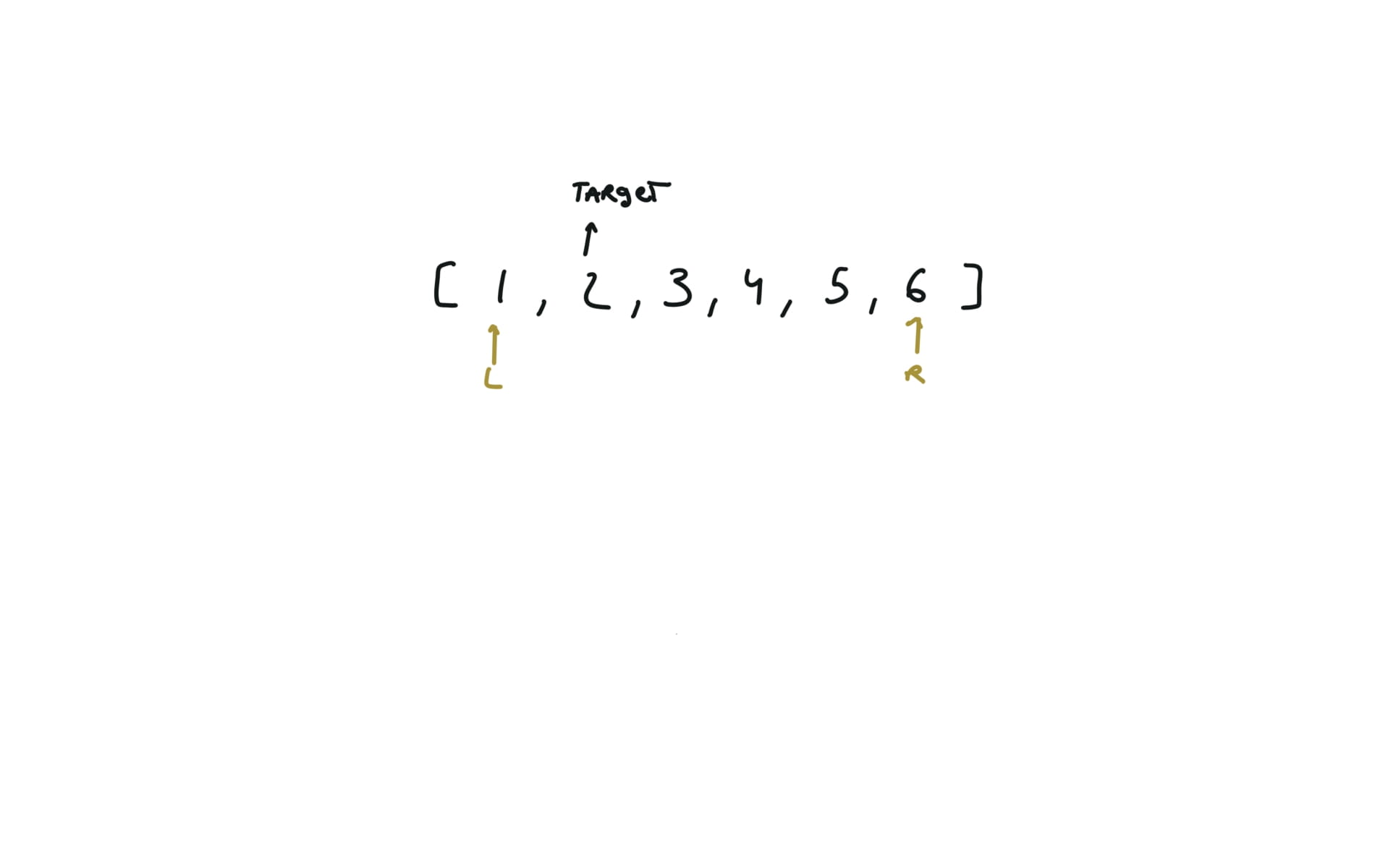
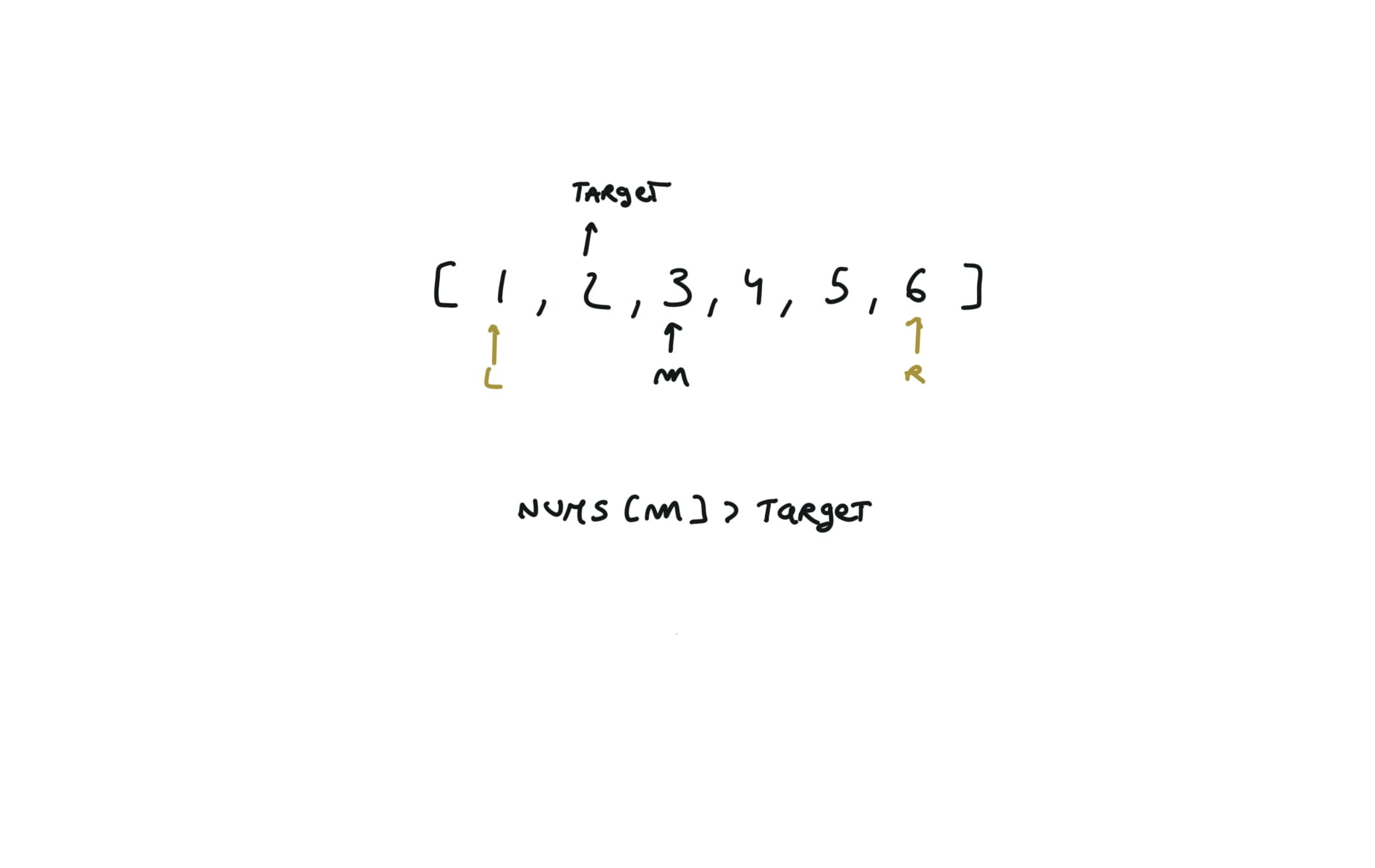
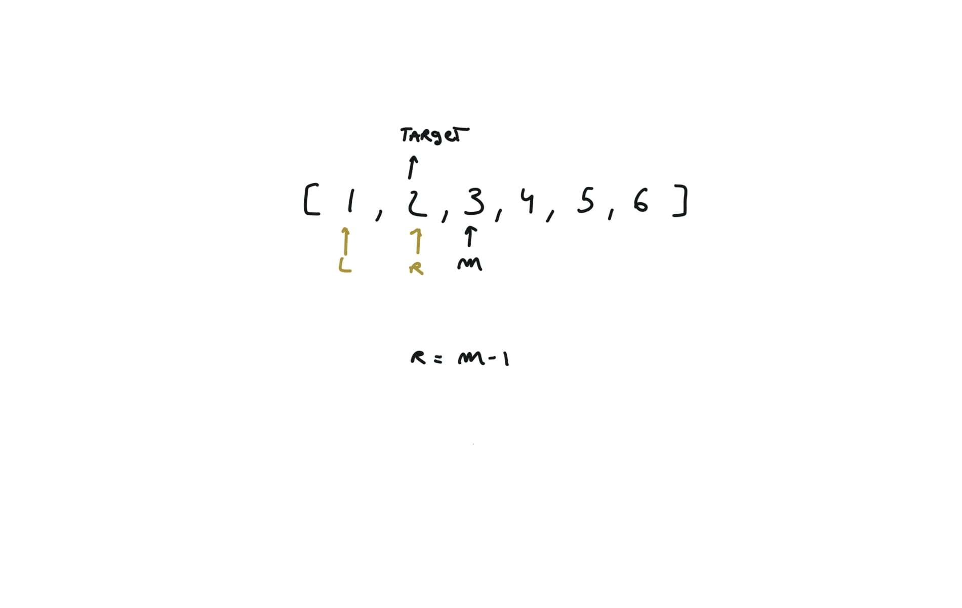
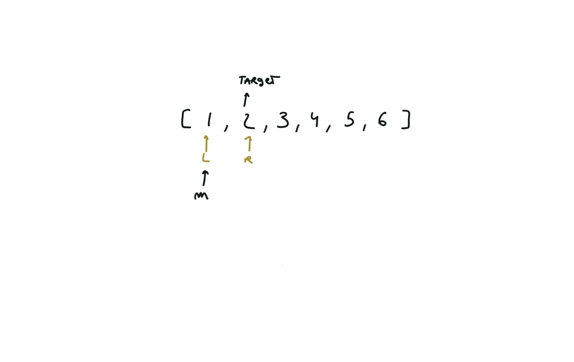
l,r = 0,len(nums)-1
while l<=r:
    m = (l+r) // 2
    if nums[m] == target:
        return m
    if nums[m] > target:
        r = m - 1
    else:
        l = m + 1
return -1
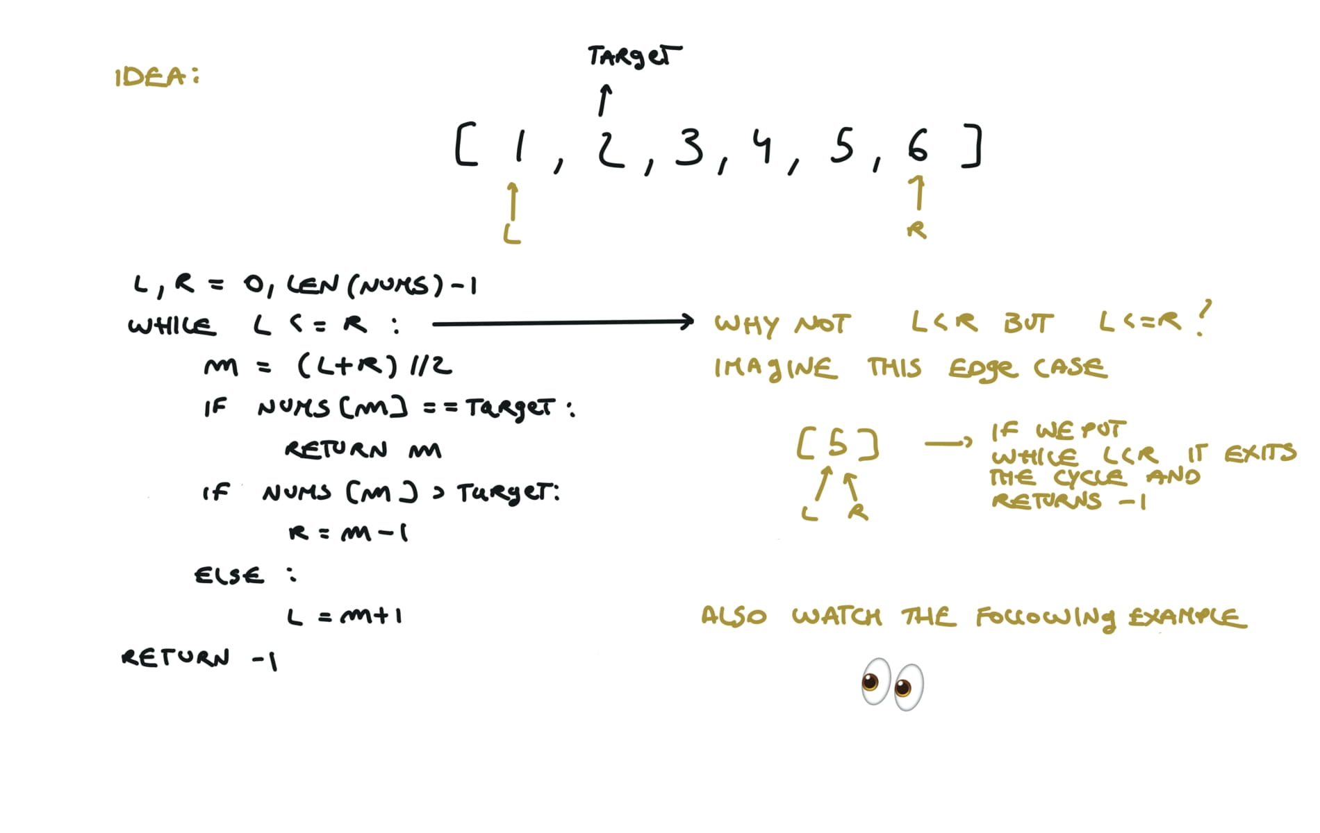
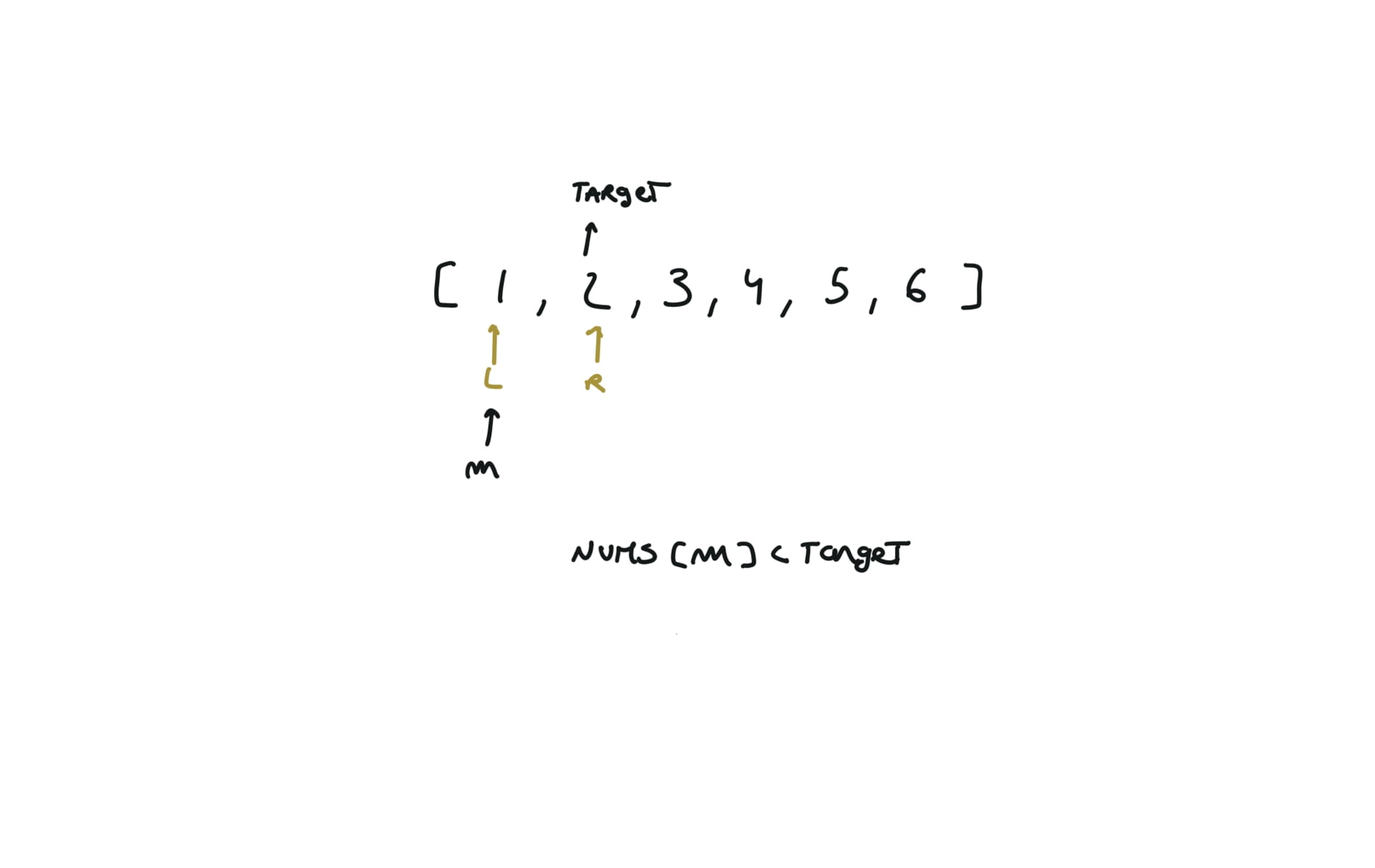
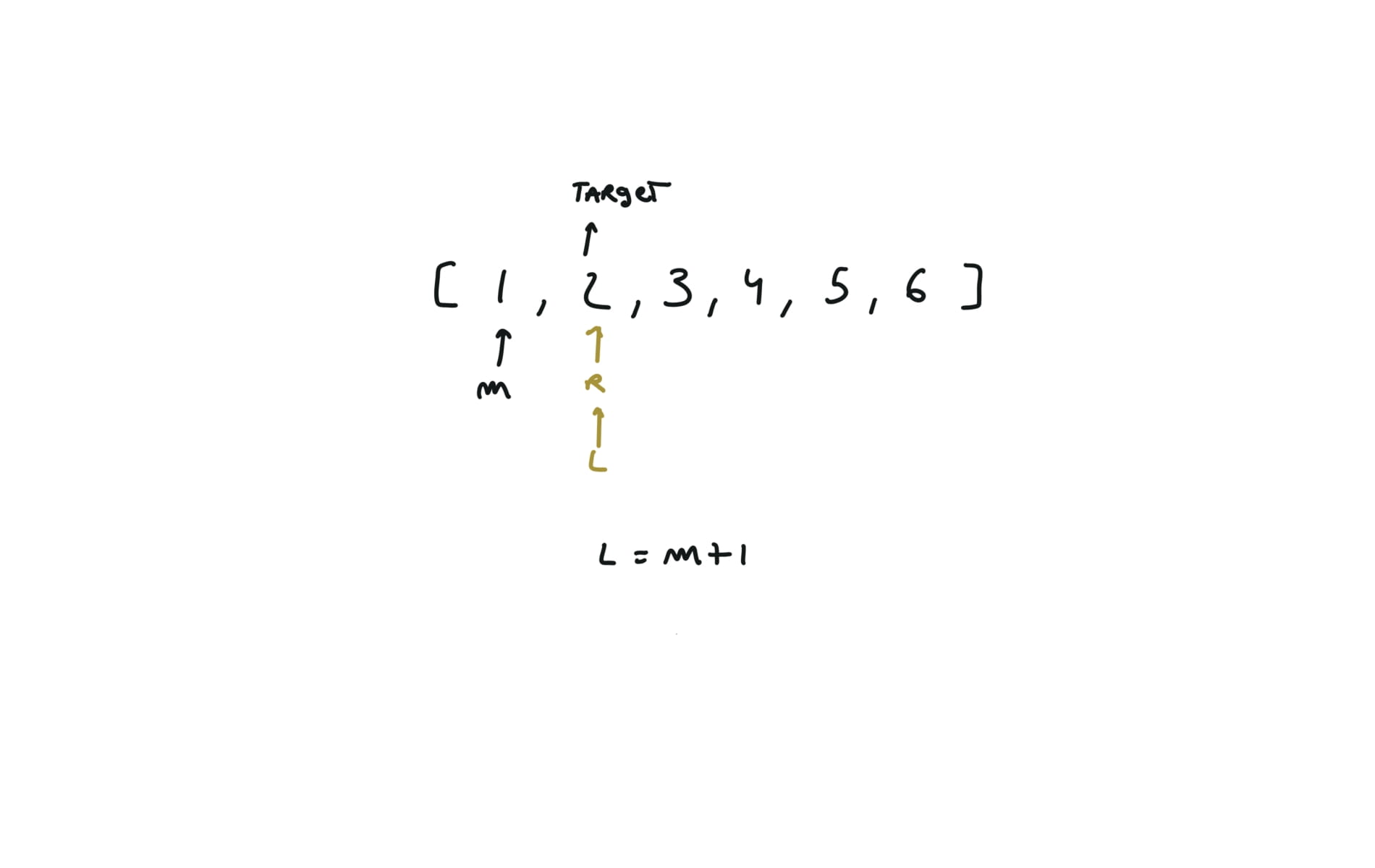
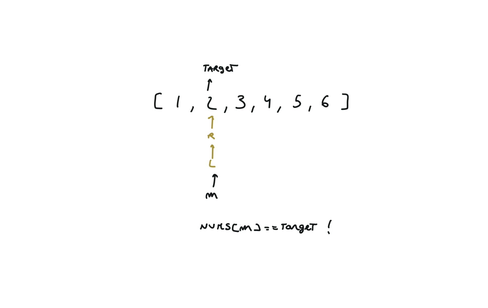
visualization
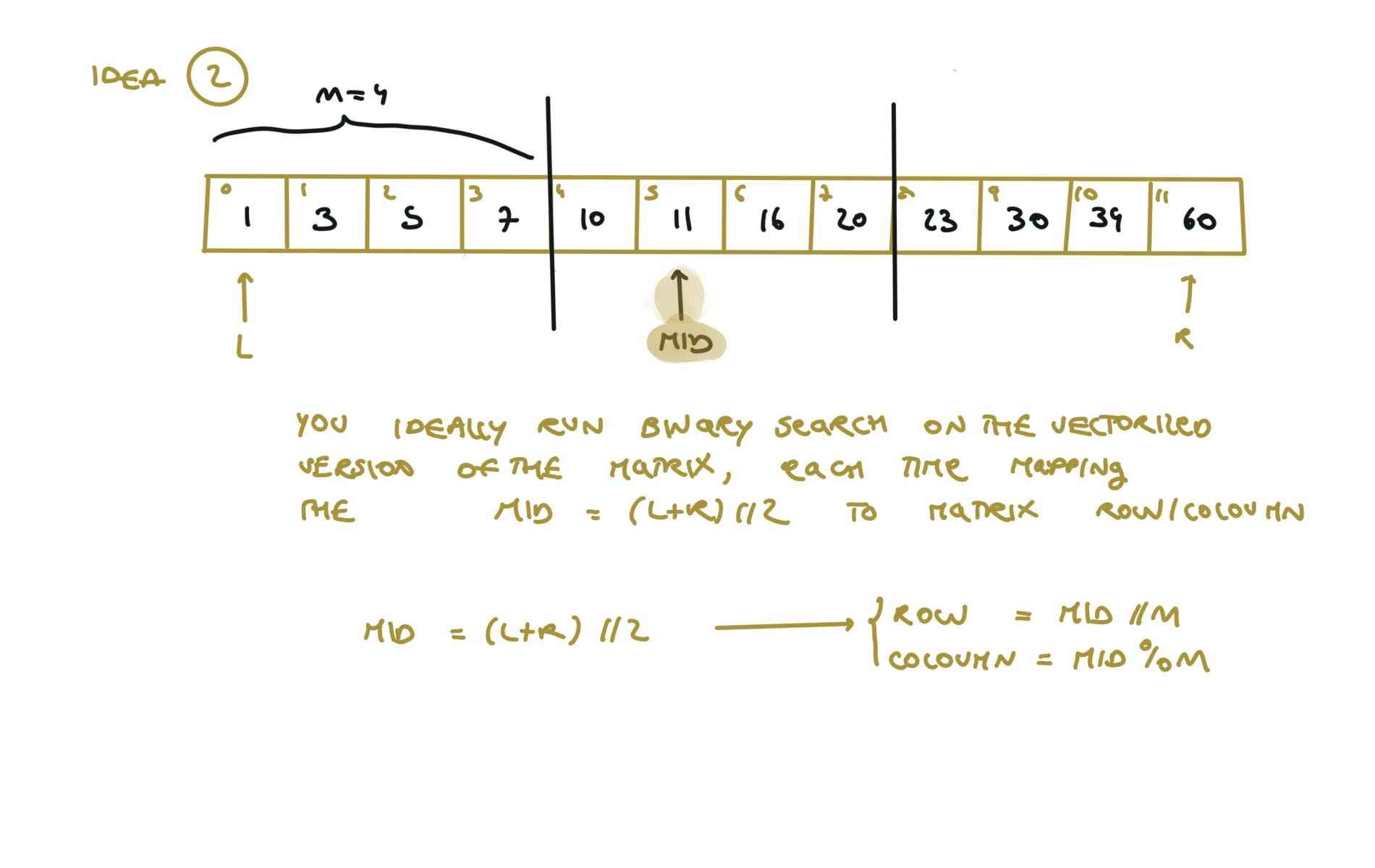
74. Search a 2D Matrix
[desc]
(link)
m = len(matrix)
n = len(matrix[0])
left, right= 0, m*n-1
while left <= right:
    mid = (left + right) // 2
    mid_row, mid_col = mid // n, mid % n
    if matrix[mid_row][mid_col] == target:
        return True
    elif matrix[mid_row][mid_col] < target:
        left = mid + 1
    else:
		right = mid - 1
return False
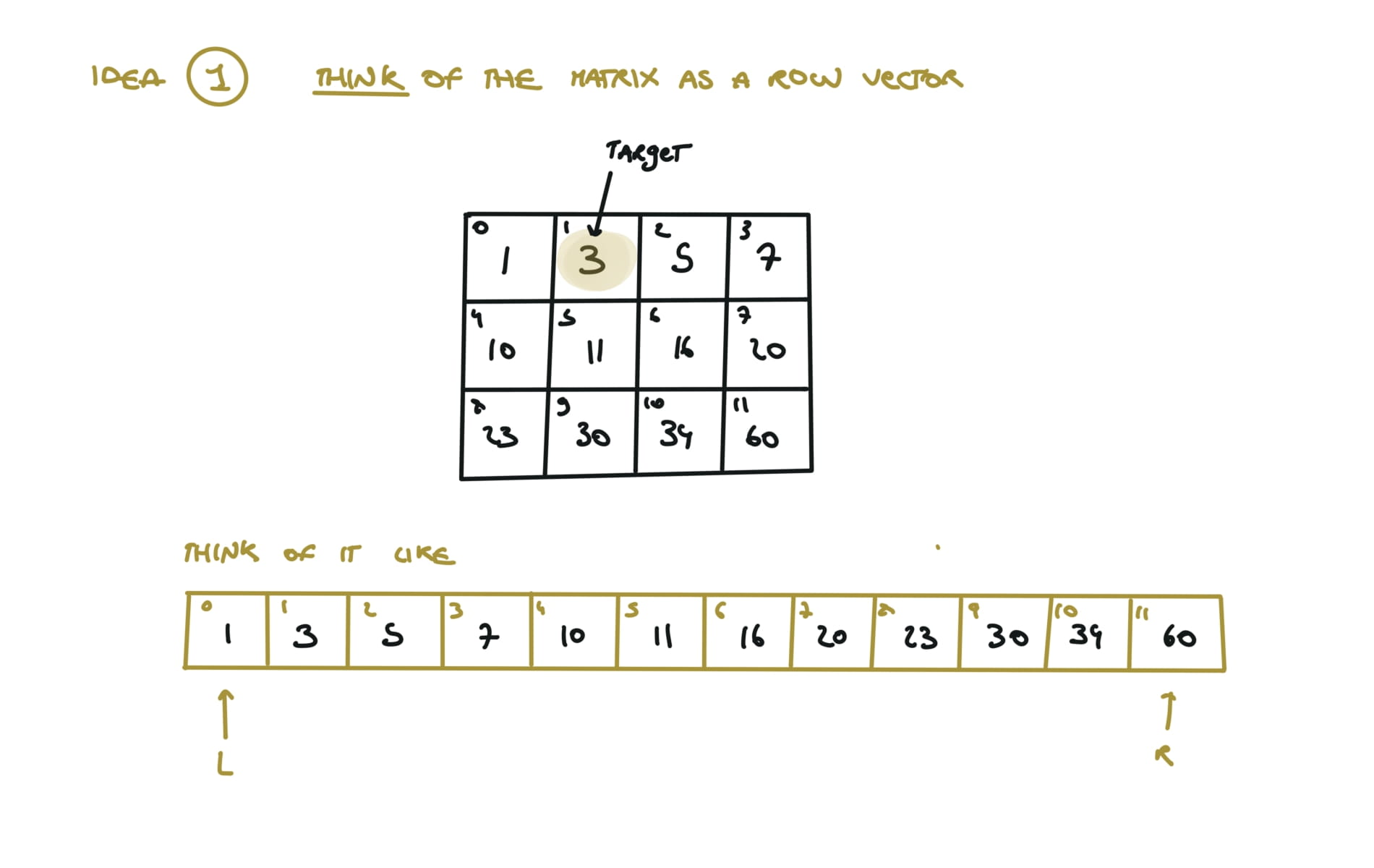
visualization
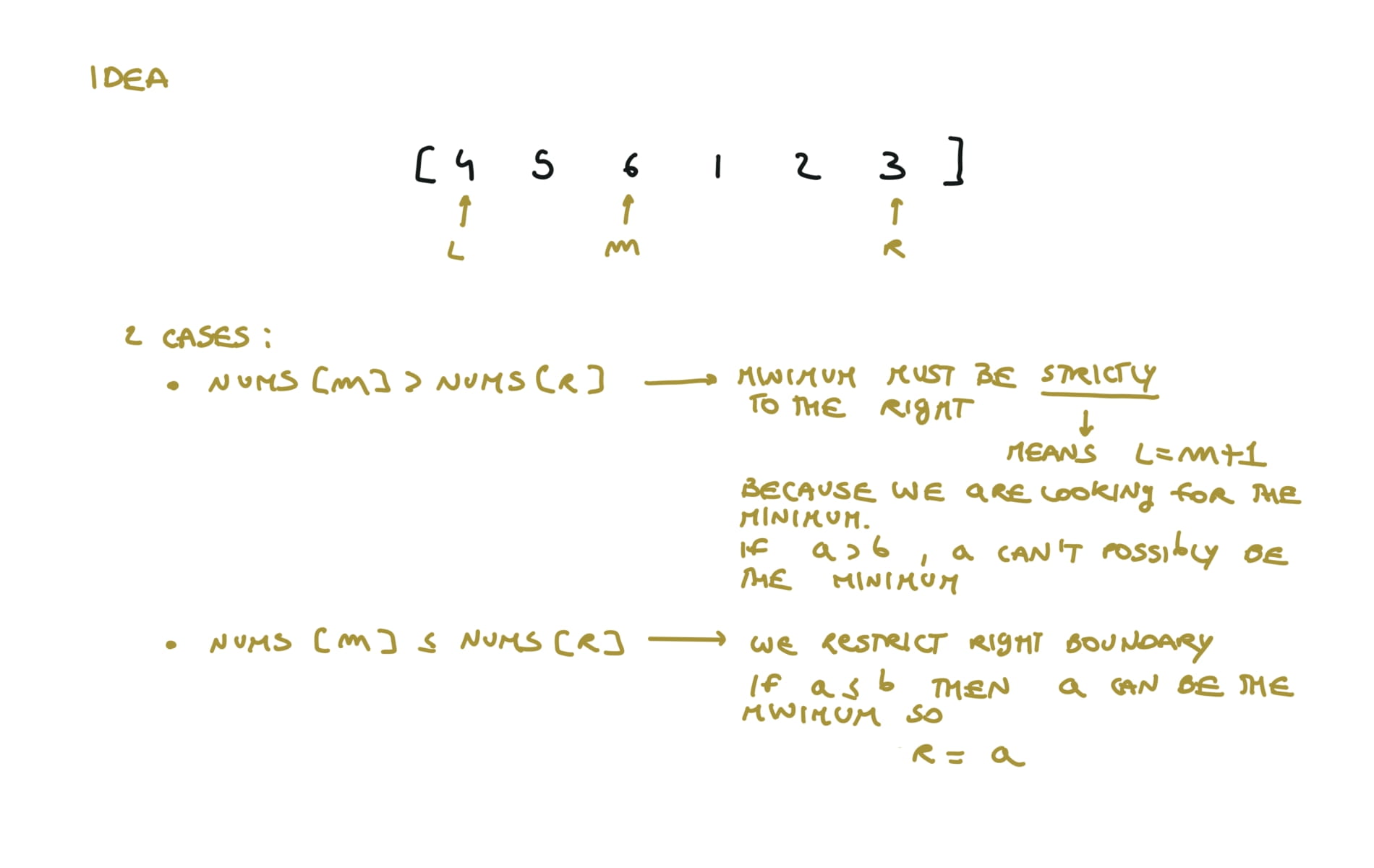
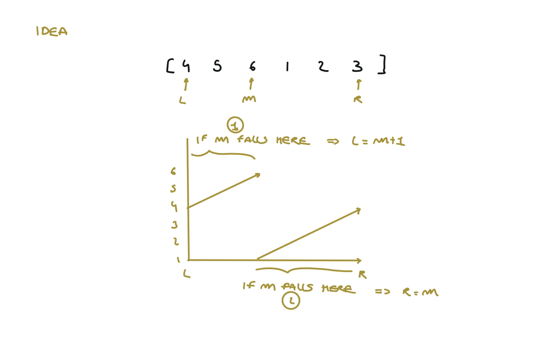
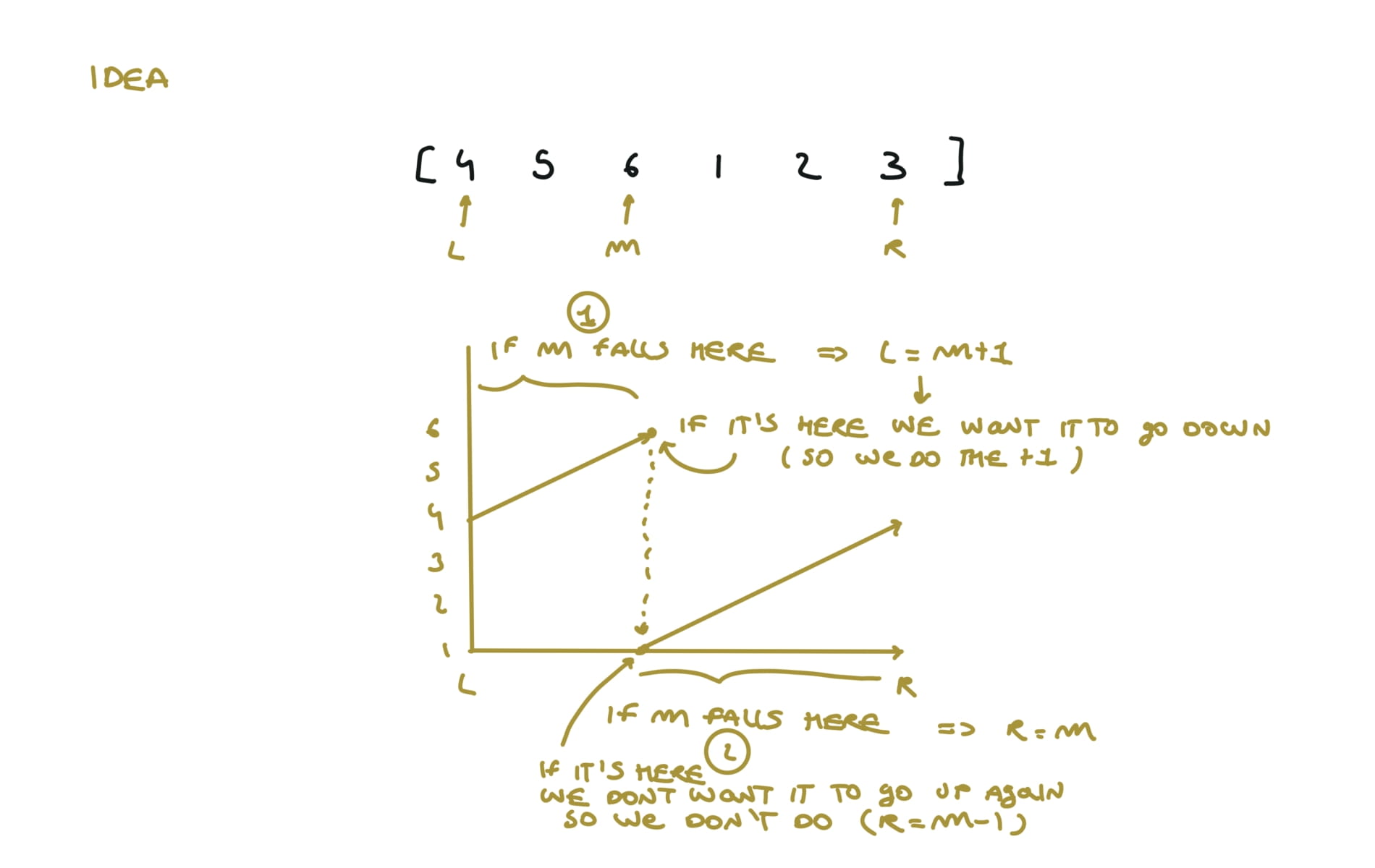
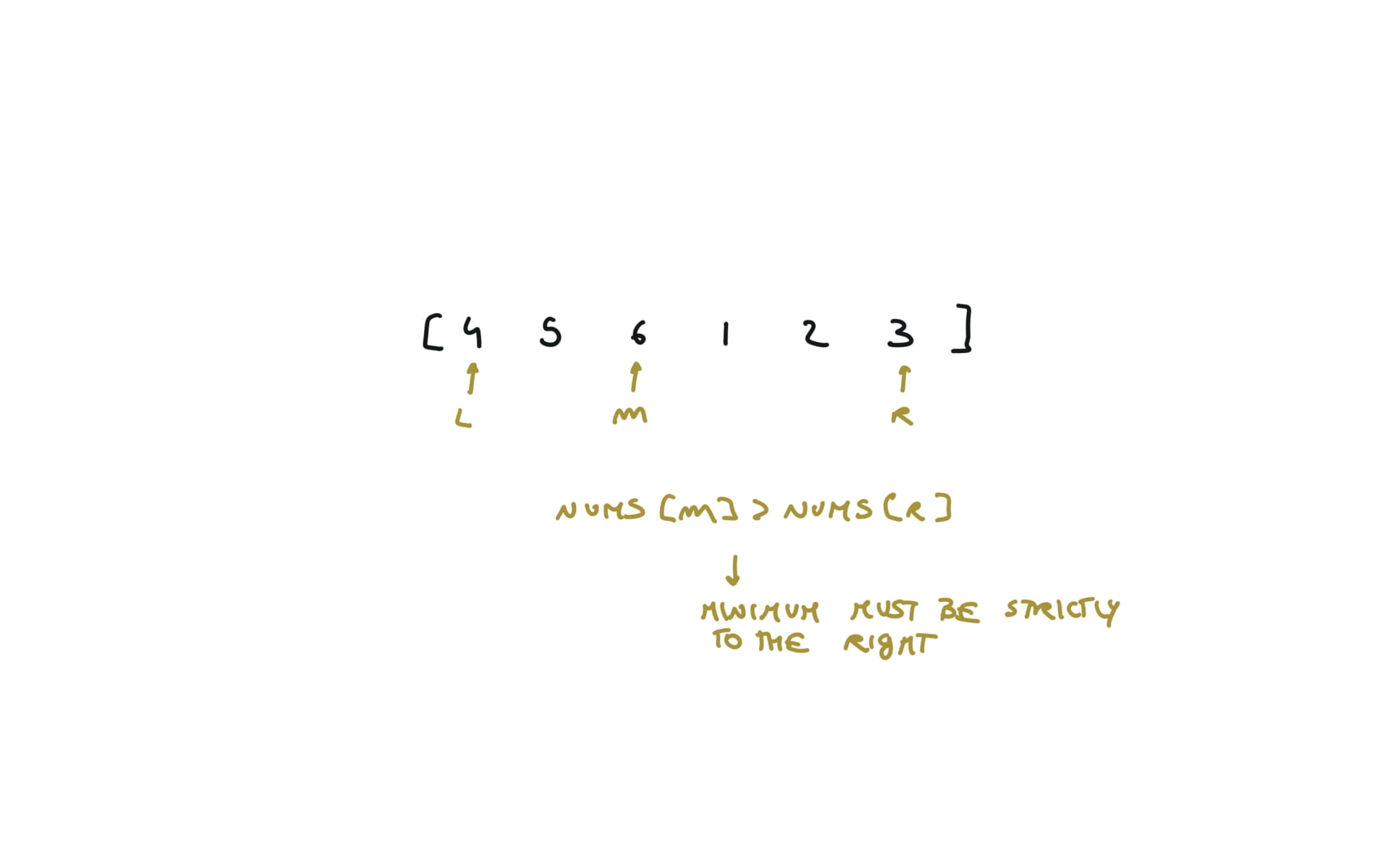
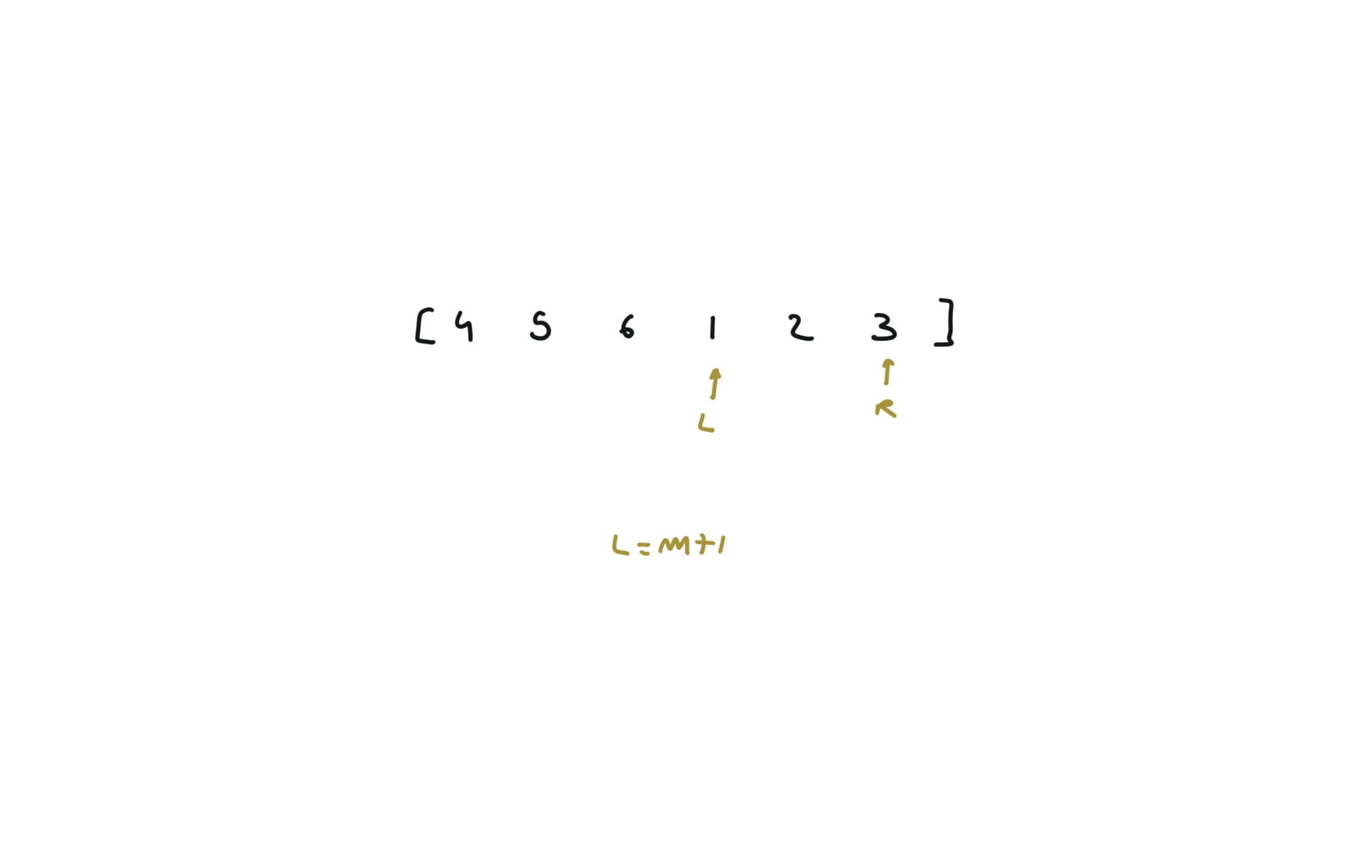
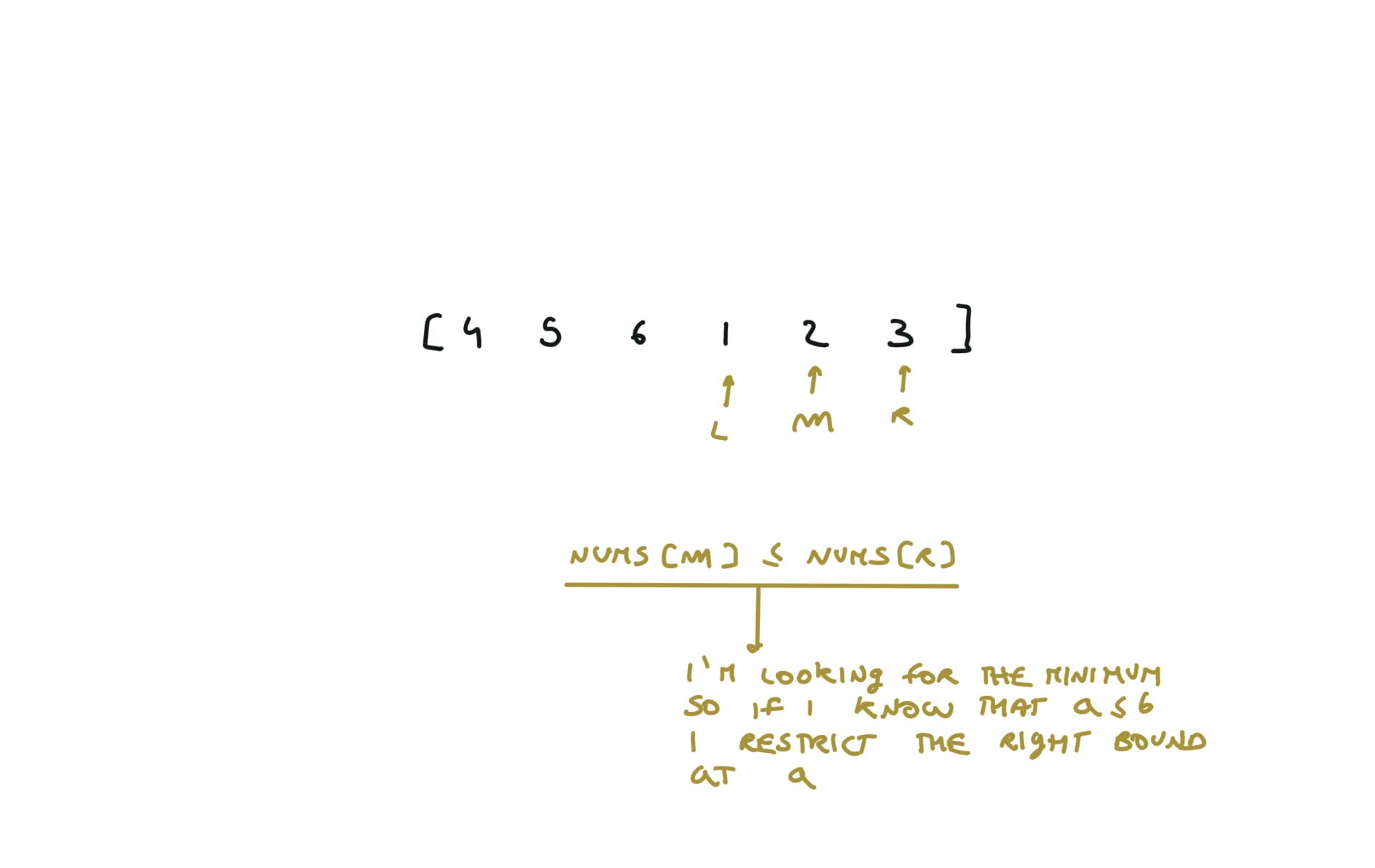
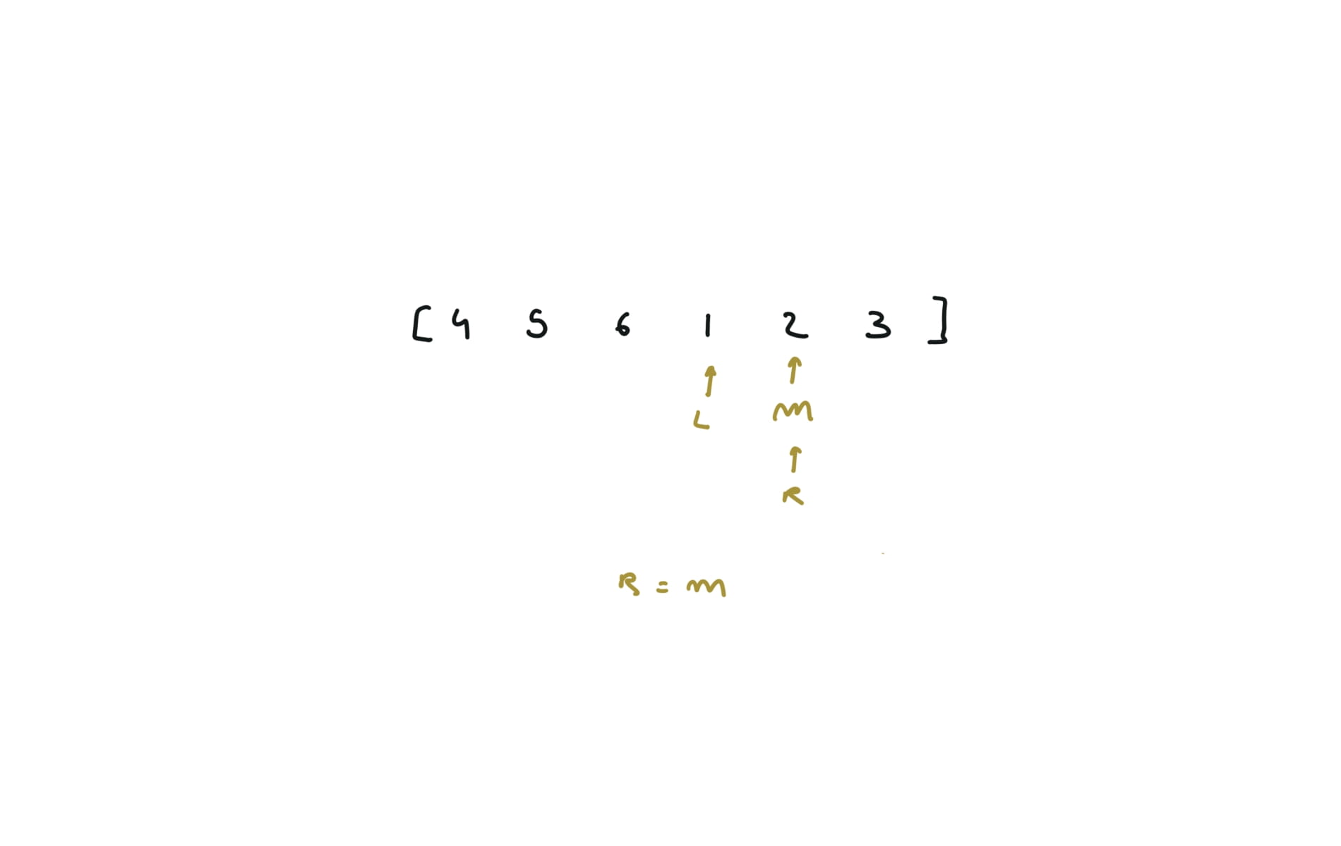
153. Find Minimum in Rotated Sorted Array
[desc]
(link)
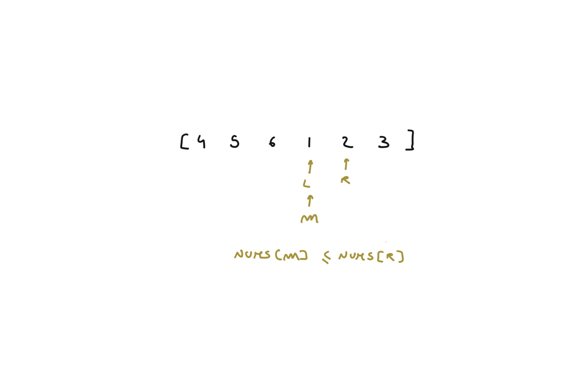
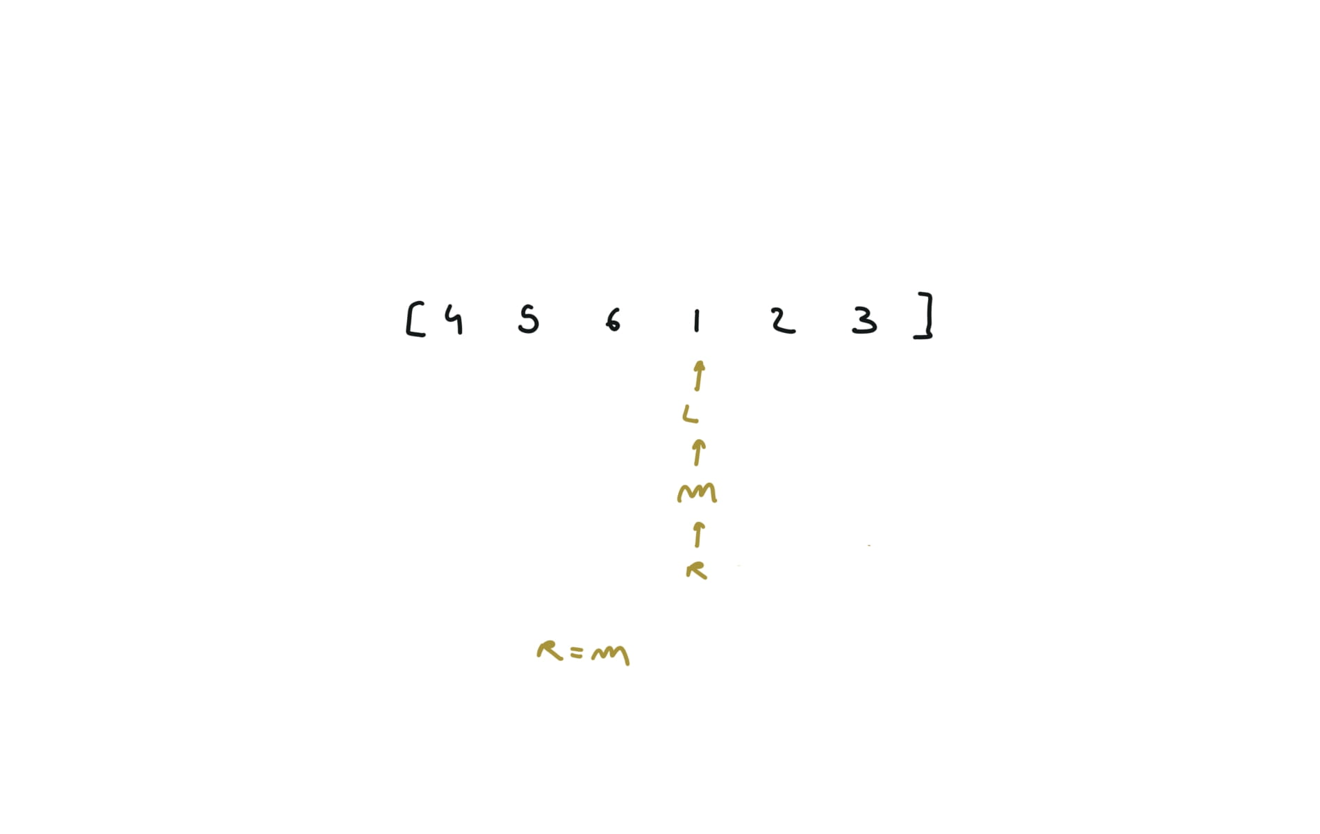
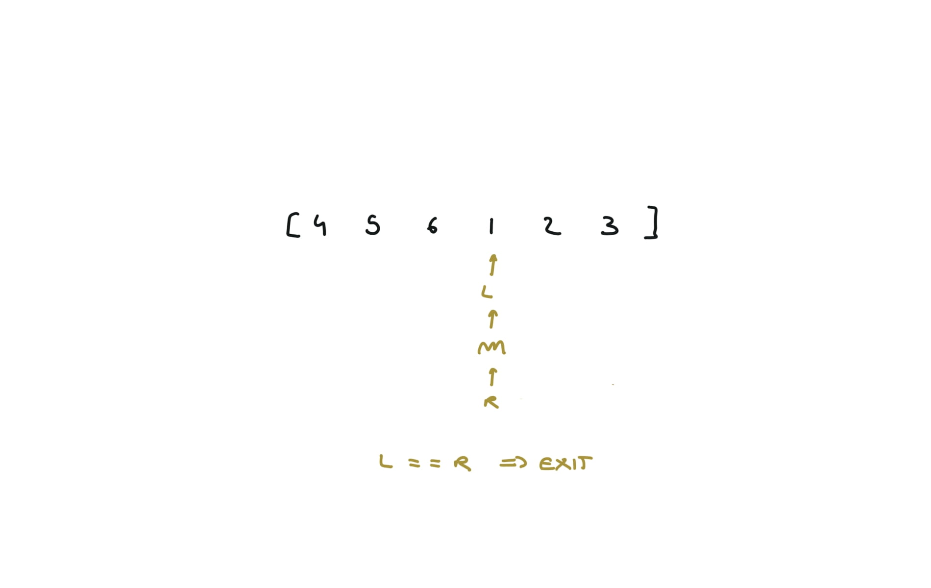
l, r = 0,len(nums)-1
while l < r:
    m = (l+r) // 2
    if nums[m] > nums[r]:
        l = m+1
    else:
        r = m
return nums[l]
visualization
33. Search in Rotated Sorted Array
[desc]
(link)
l,r = 0,len(nums)-1
while l <= r:
    m = (l+r) //2
    if nums[m] == target:
        return m
    if nums[l] <= nums[m]: #left half is sorted
        if nums[l] <= target <= nums[m]:
            r = m-1
        else:
            l = m+1
    else:
        if nums[m] <= target <= nums[r]:
            l = m+1
        else:
            r = m-1
return -1
Linked list
206. Reverse Linked List
[desc]
(link)
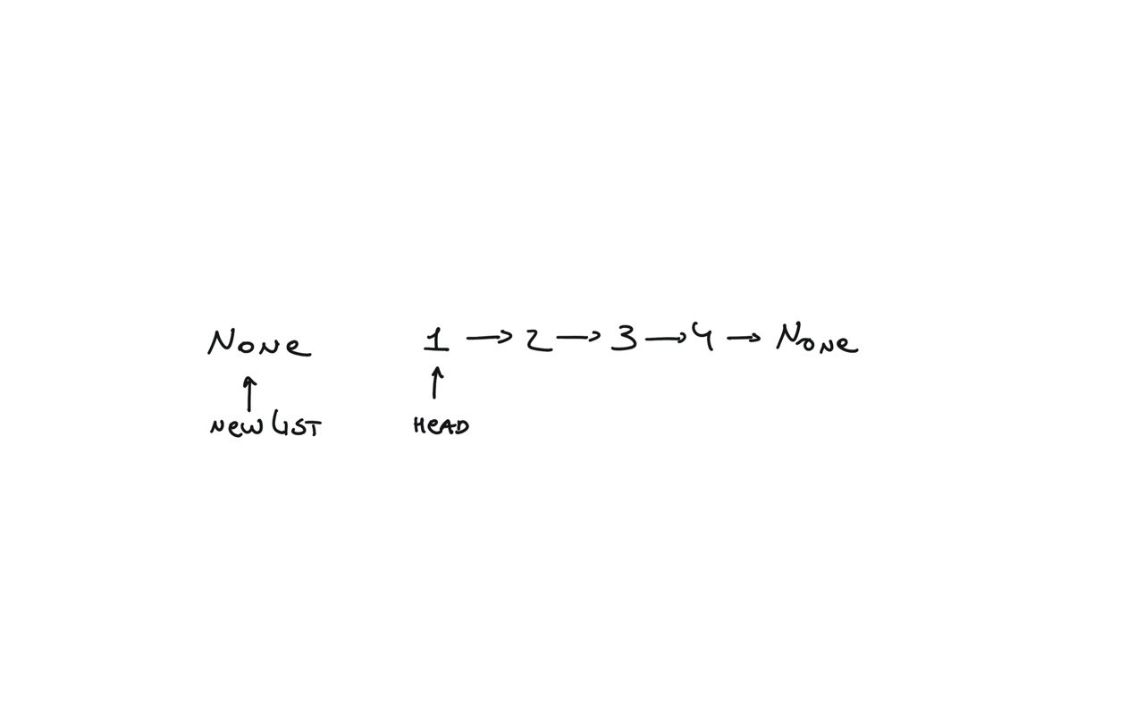
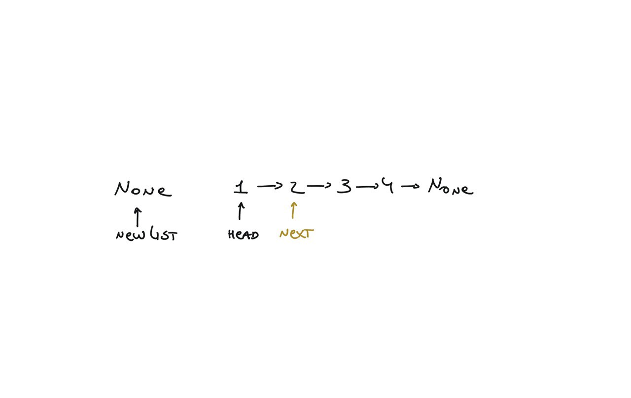
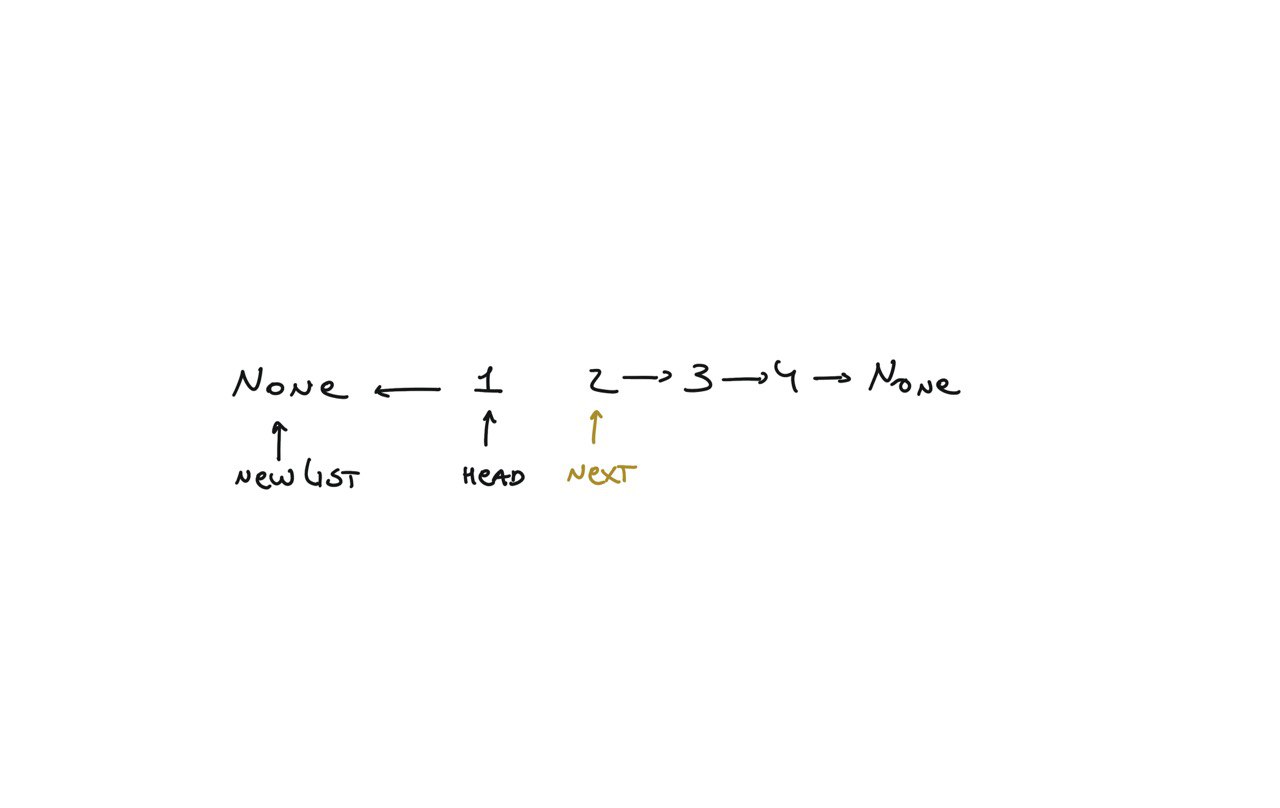
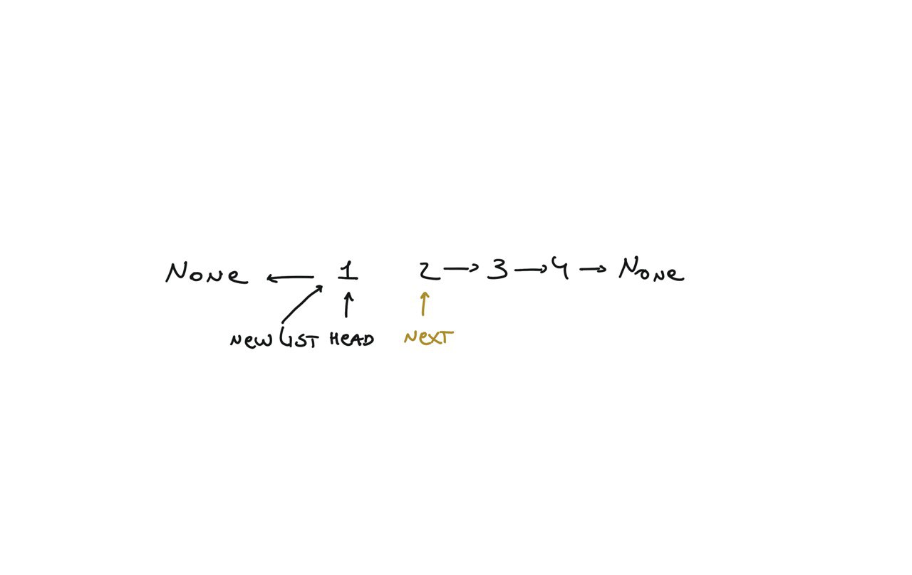
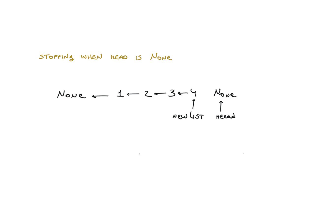
newList = None
while head:
	next = head.next
	head.next = newList
	newList = head
	head = next
return newList
visualization
21. Merge Two Sorted Lists
[desc]
(link)
newList = ListNode()
tail = newList
while list1 != None and list2 != None:
    if list1.val < list2.val:
        tail.next = list1
        list1 = list1.next
    else:
        tail.next = list2
        list2 = list2.next
        tail = tail.next
    if list1 != None:
        tail.next = list1
    elif list2 != None:
        tail.next = list2
return newList.next
143. Reorder List
[desc]
(link)
# find middle
slow, fast = head, head.next
while fast and fast.next:
    slow = slow.next
    fast = fast.next.next

# reverse second half
second = slow.next
prev = slow.next = None
while second:
    tmp = second.next
    second.next = prev
    prev = second
    second = tmp

# merge two halfs
first, second = head, prev
while second:
    tmp1, tmp2 = first.next, second.next
    first.next = second
    second.next = tmp1
    first, second = tmp1, tmp2
19. Remove Nth Node From End of List
[desc]
(link)
dummyNode = ListNode()
dummyNode.next = head
l = dummyNode
i = 0
r = dummyNode.next
while i < n:
    r = r.next
    i += 1

while r:
    l = l.next
    r = r.next

l.next = l.next.next
return dummyNode.next
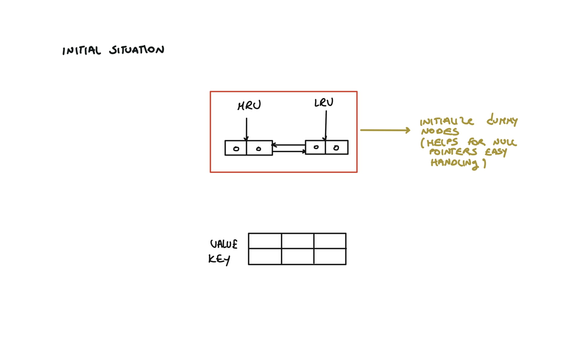
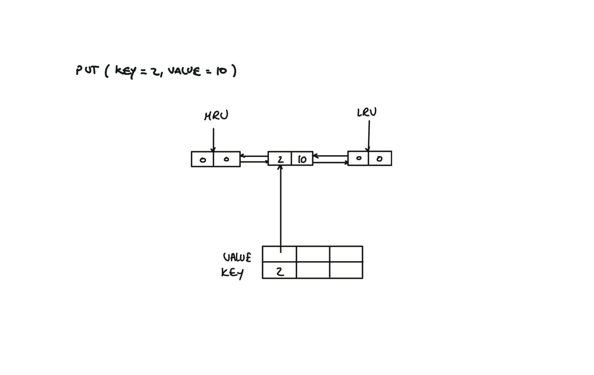
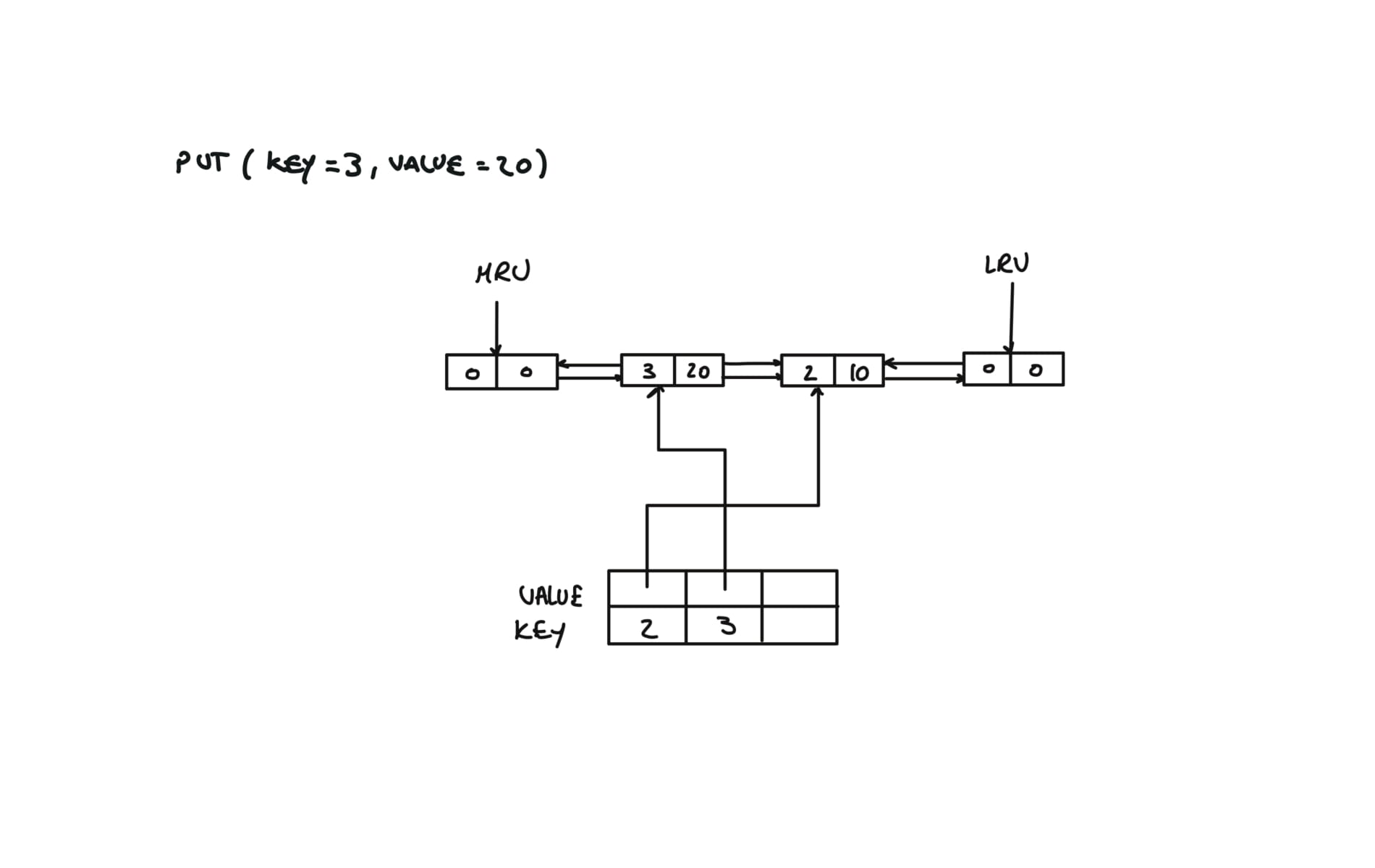
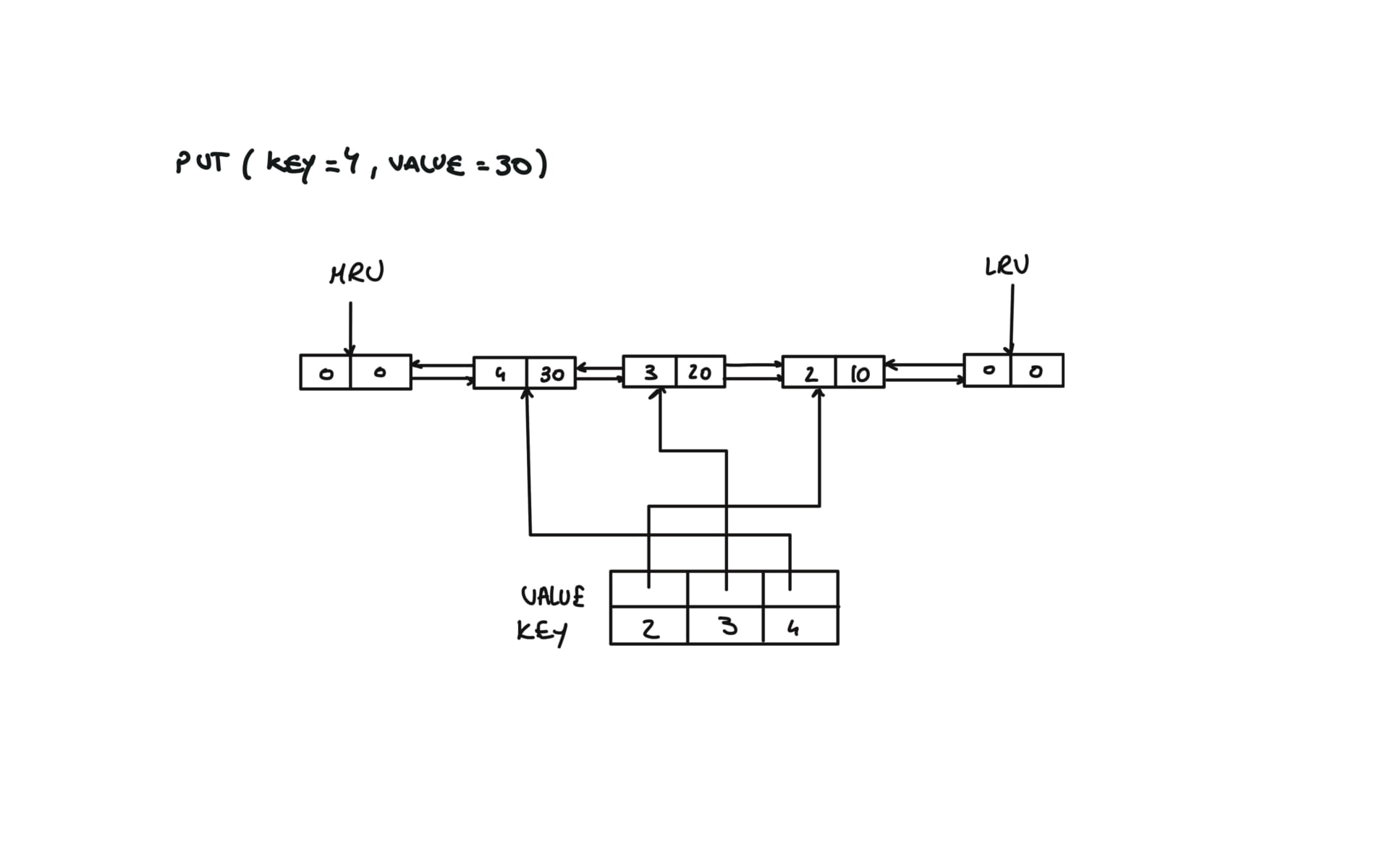
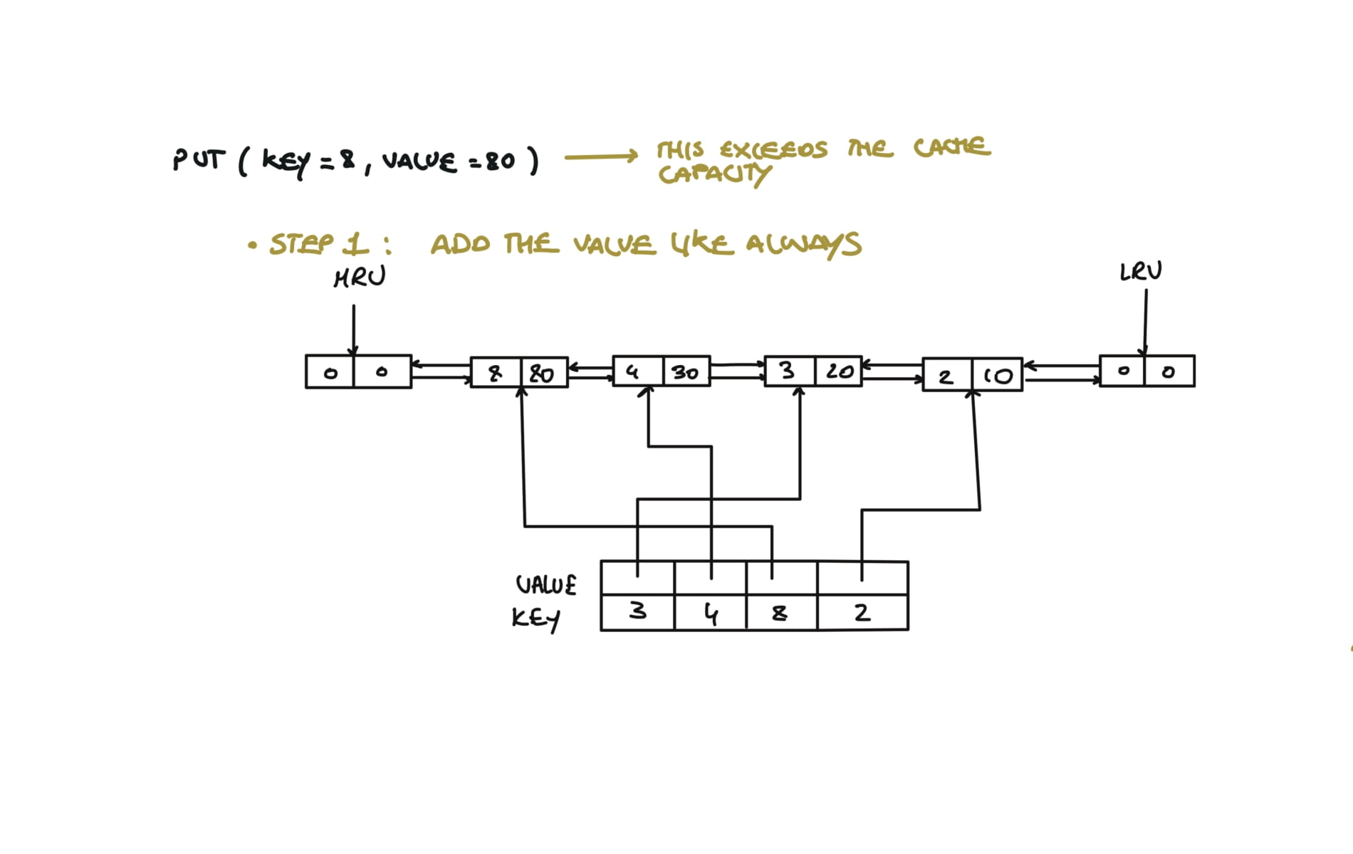
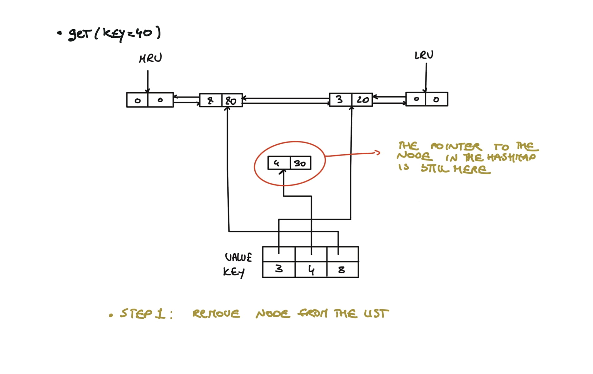
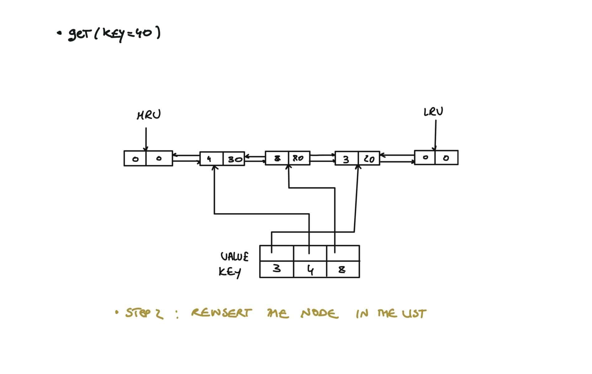
146. LRU Cache
[desc]
(link)
class LRUCache:

    def __init__(self, capacity: int):
        self.capacity = capacity
        self.cache = {}
        self.lru = Node(0,0)
        self.mru = Node(0,0)
        self.lru.next = self.mru
        self.mru.prev =  self.lru

    def get(self, key: int) -> int:
        if key in self.cache:
            self.remove(self.cache[key])
            self.insert(self.cache[key])
            return self.cache[key].value
        return -1

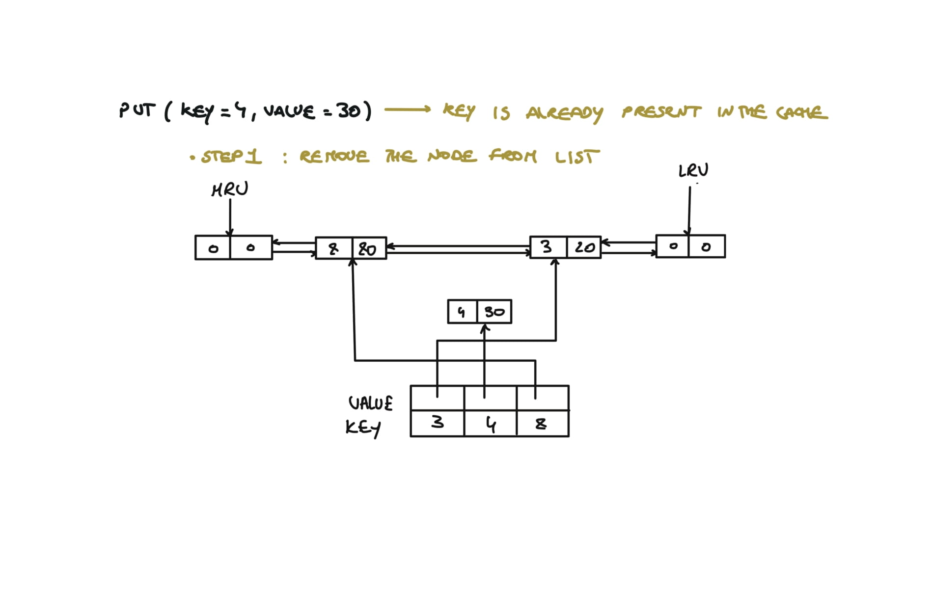
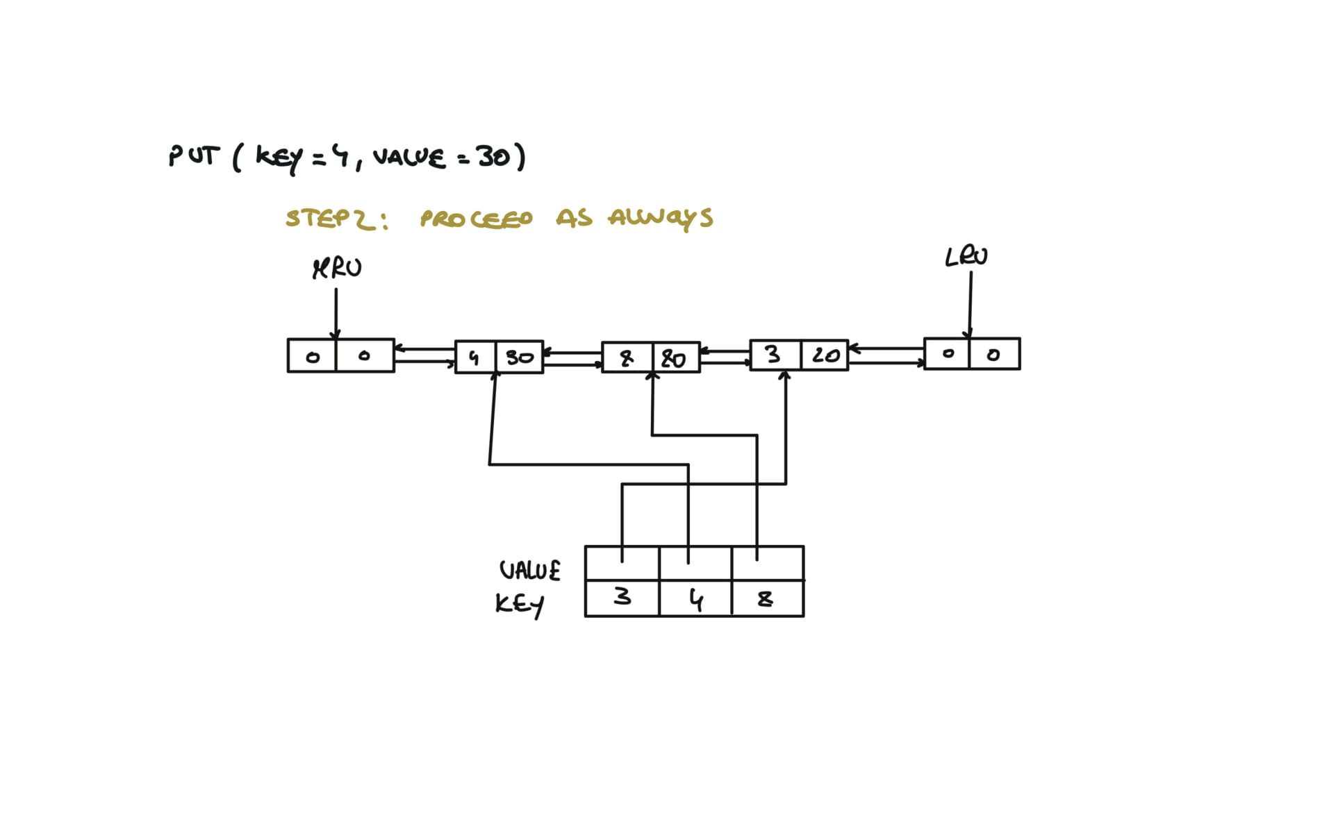
    def put(self, key: int, value: int) -> None:
        if key in self.cache:
            self.remove(self.cache[key])
        self.cache[key] = Node(key,value)
        self.insert(self.cache[key])

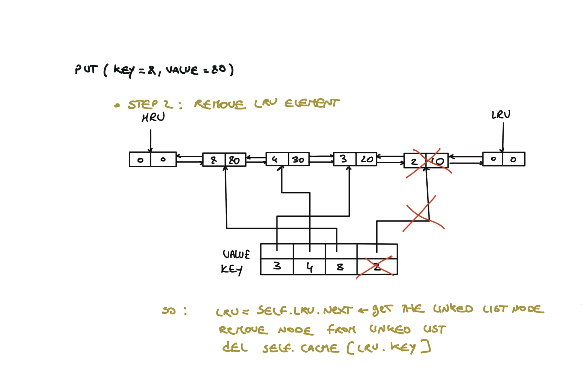
        if len(self.cache) > self.capacity:
            #remove and delete the LRU
            lru = self.lru.next
            self.remove(lru)
            del self.cache[lru.key]

	# Removes any node from linked list in O(1)
    def remove(self, node):
        prev,next = node.prev,node.next
        prev.next,next.prev = next,prev

	# Inserts new node from mru
    def insert(self,node):
        prev,next = self.mru.prev, self.mru
        prev.next = next.prev = node
        node.next, node.prev = next,prev
visualization
Trees
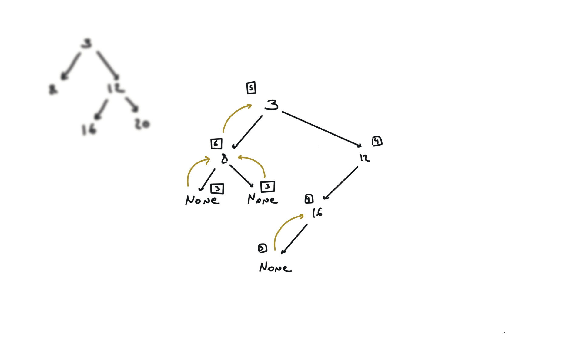
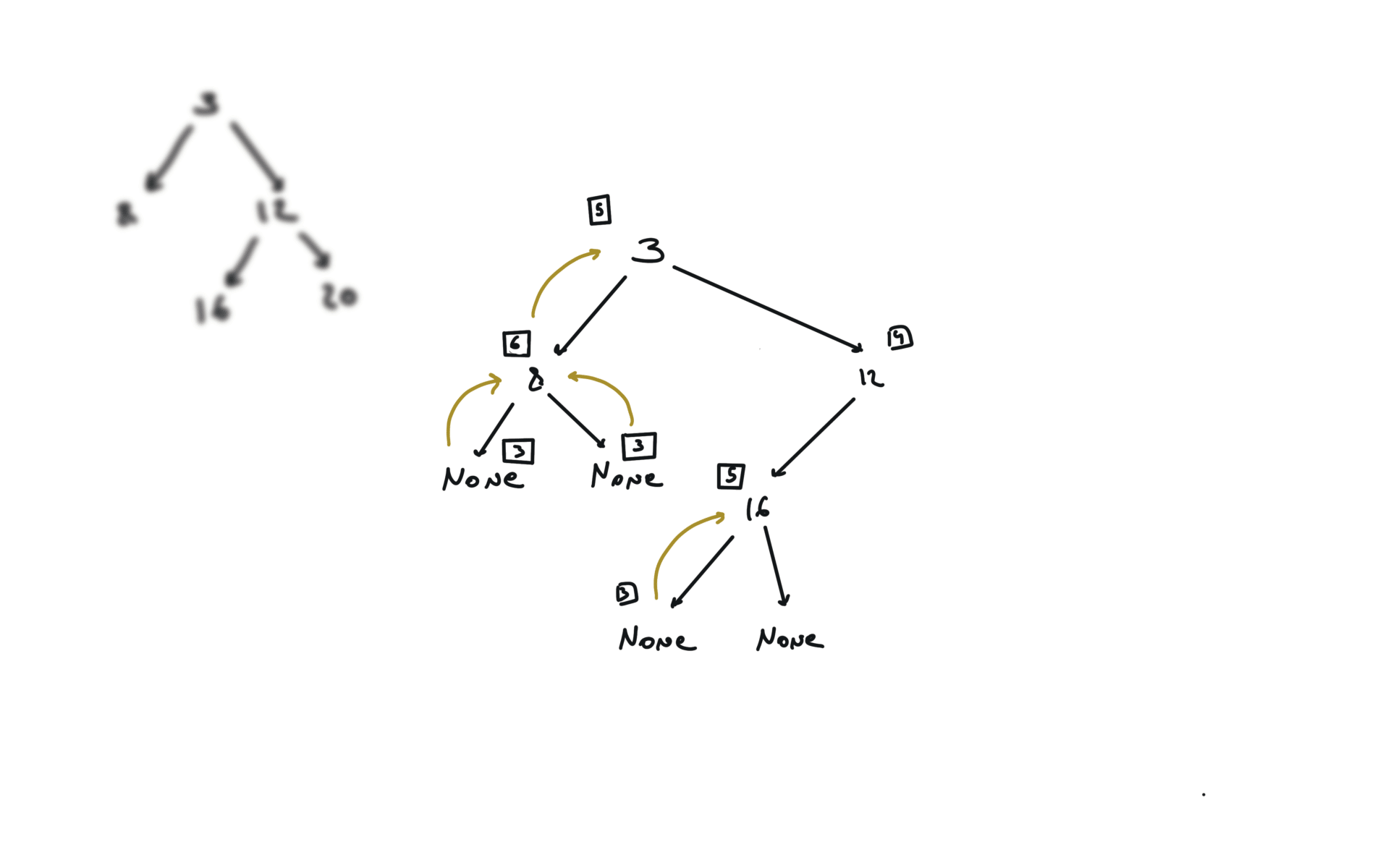
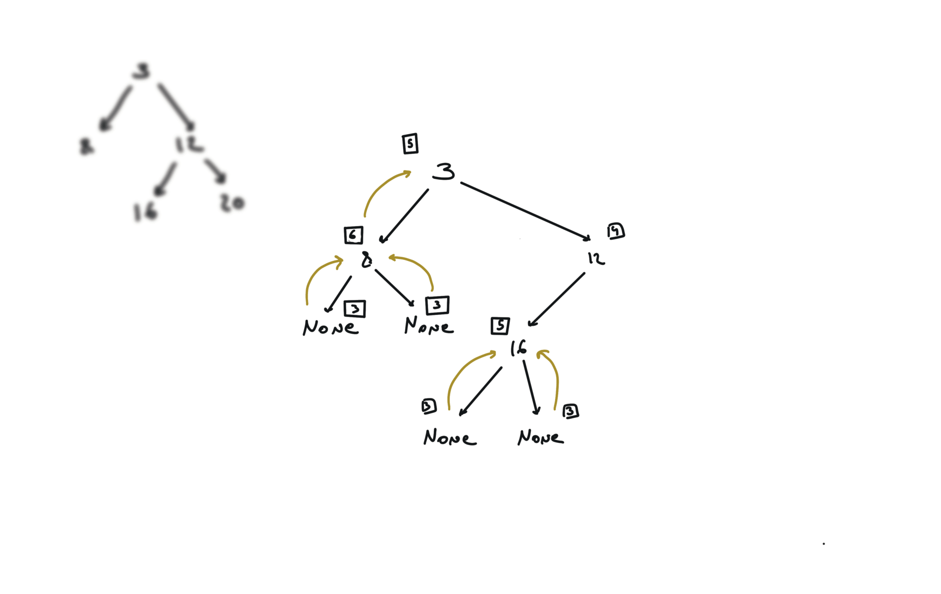
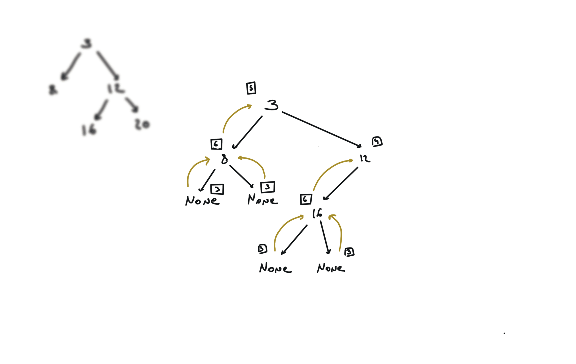
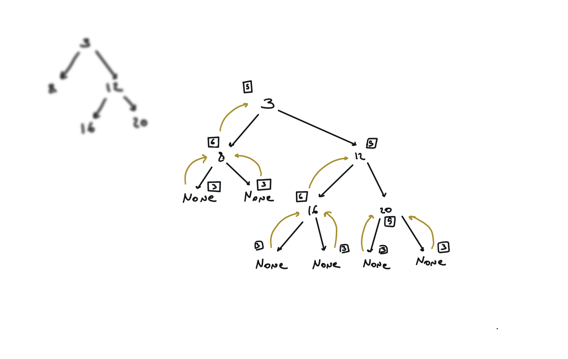
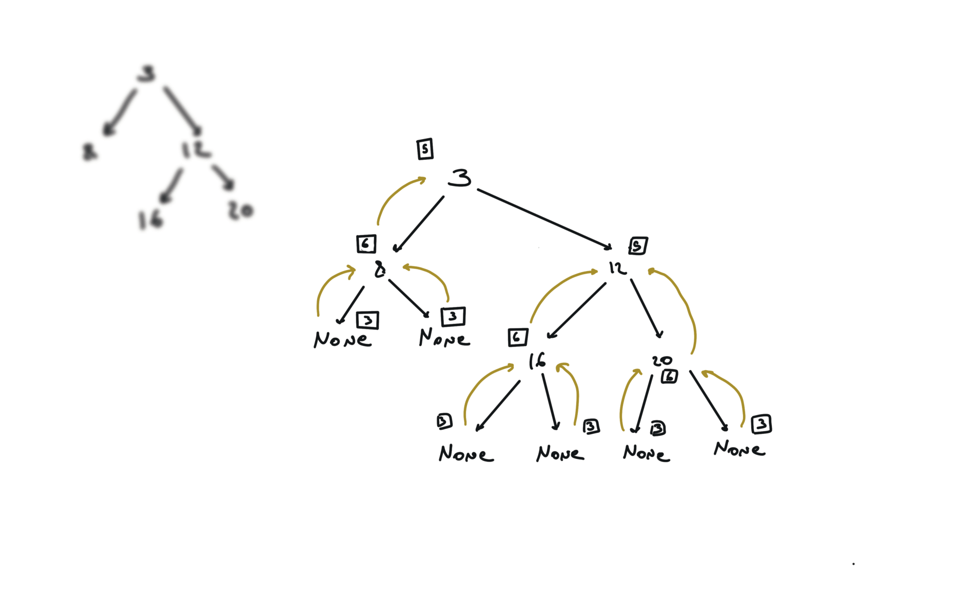
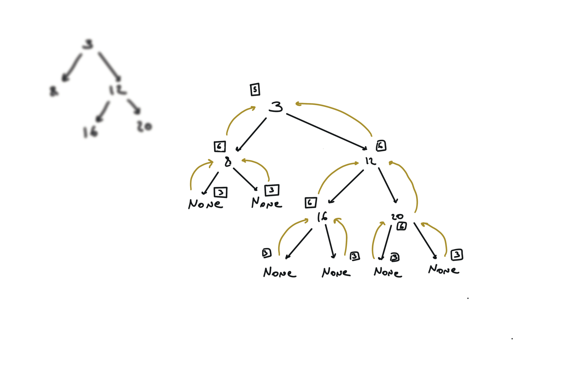
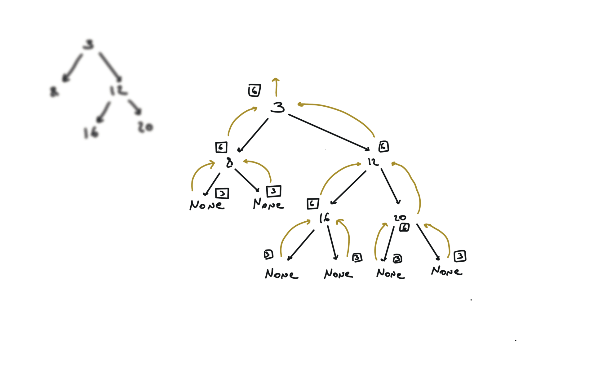
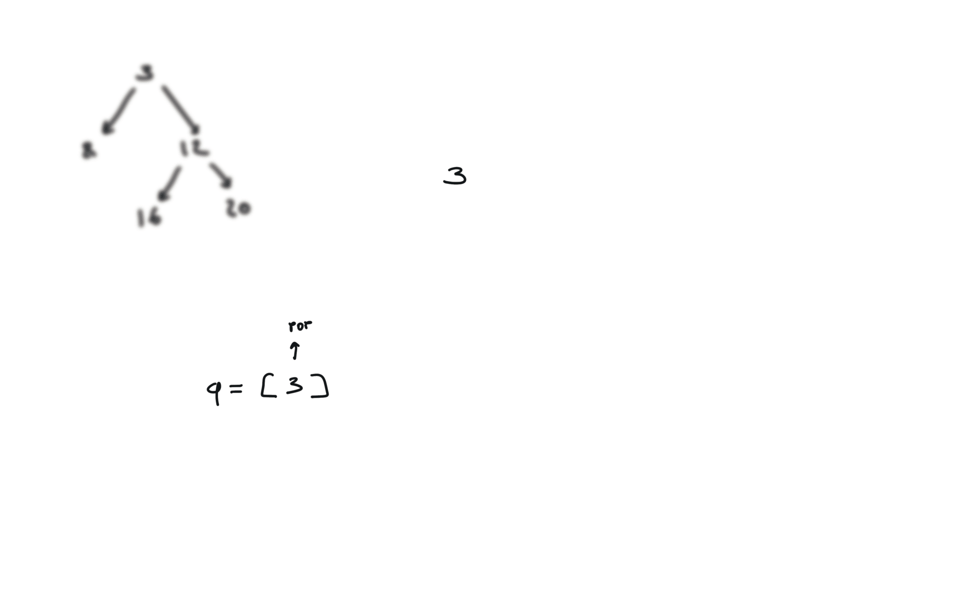
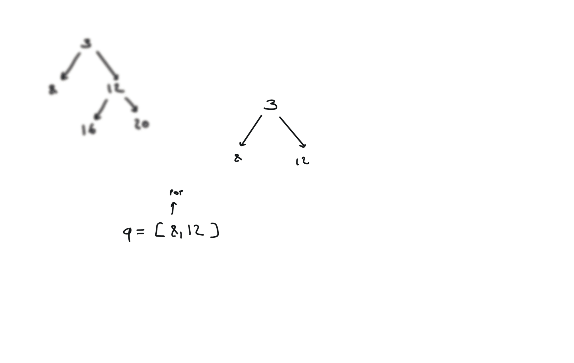
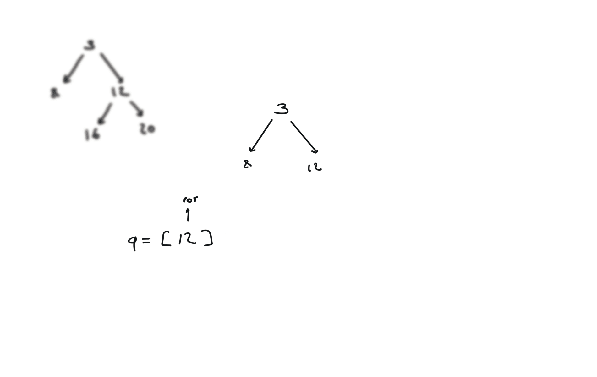
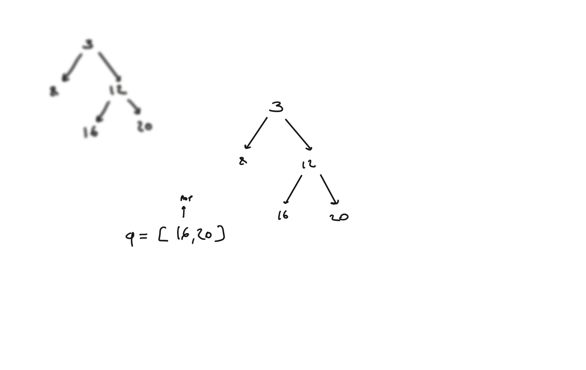
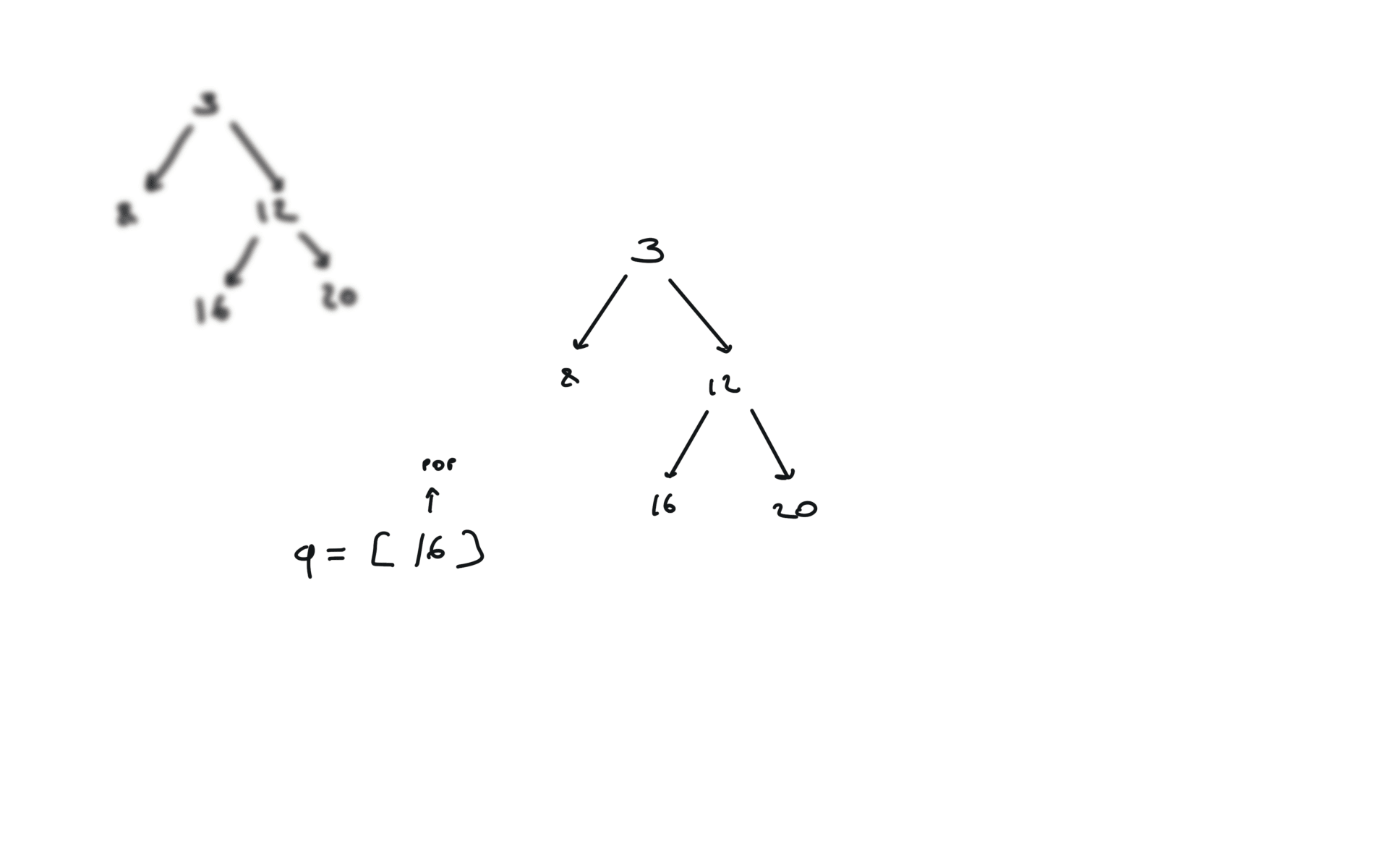
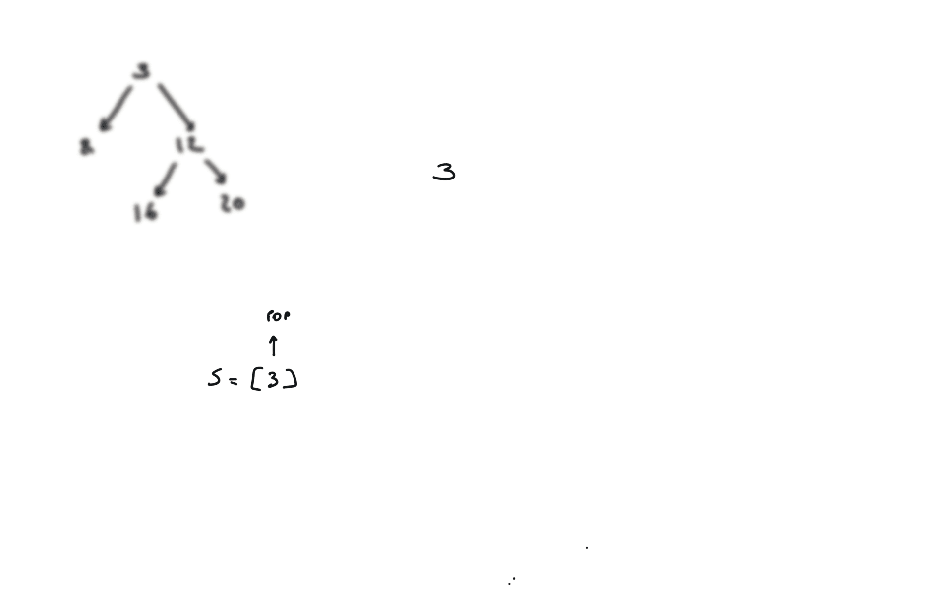
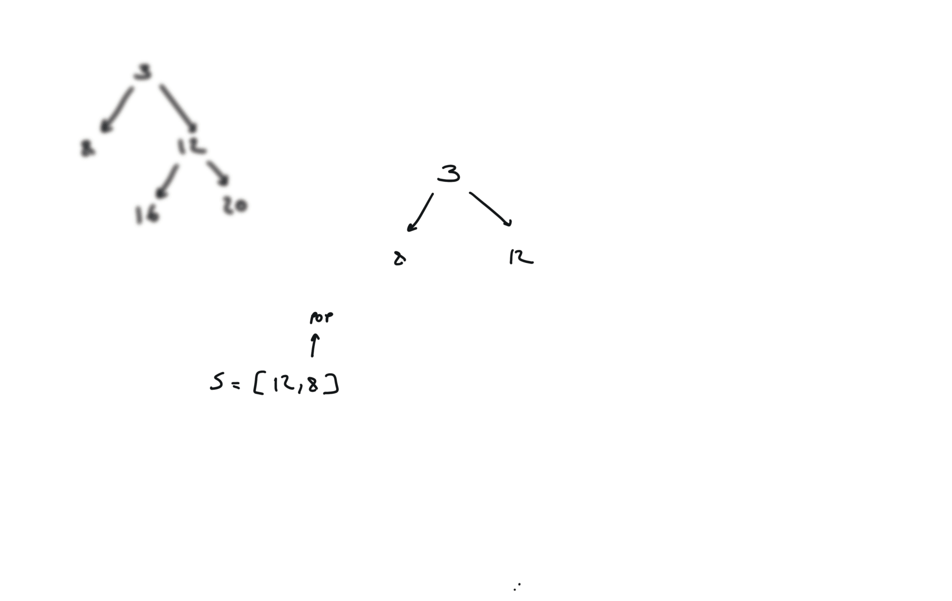
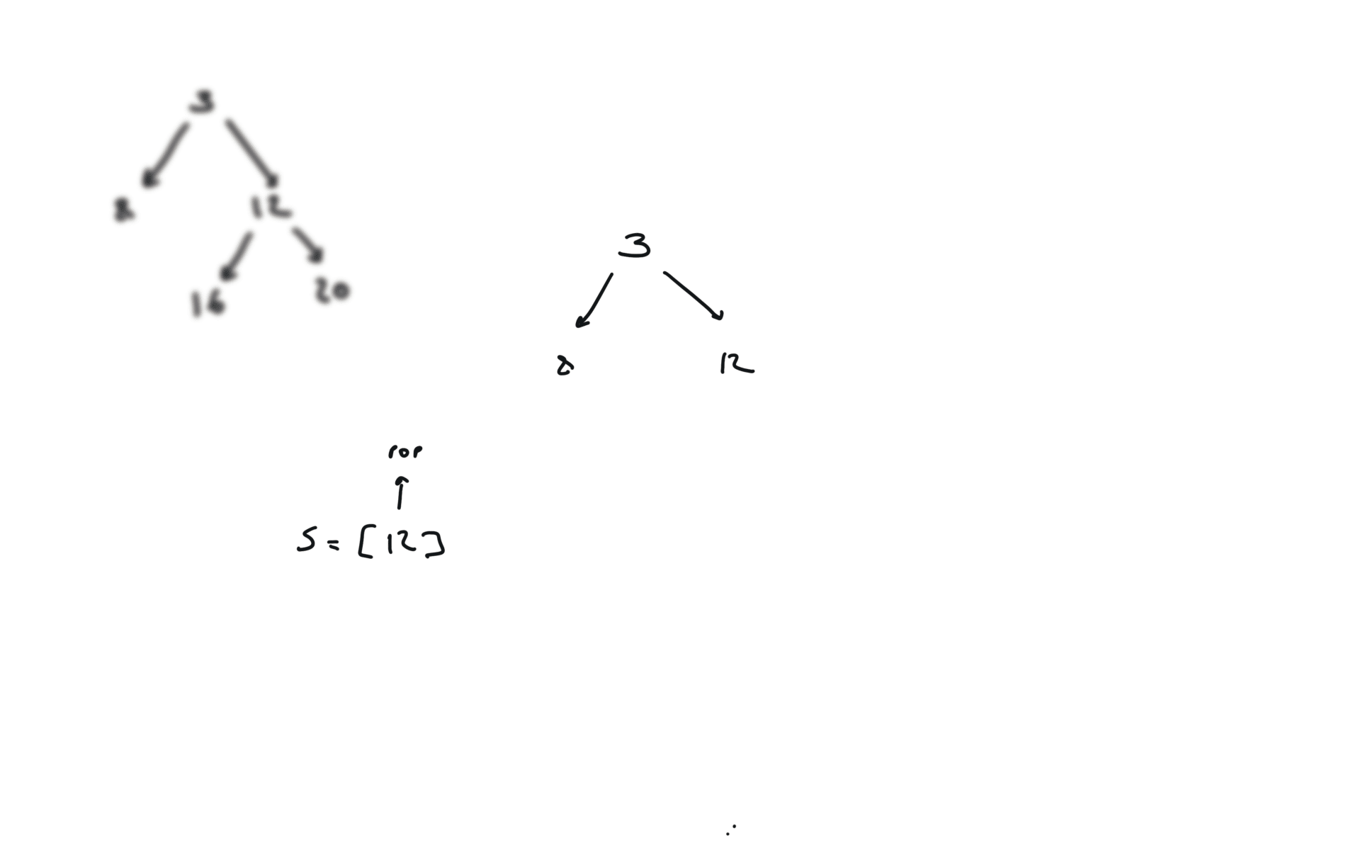
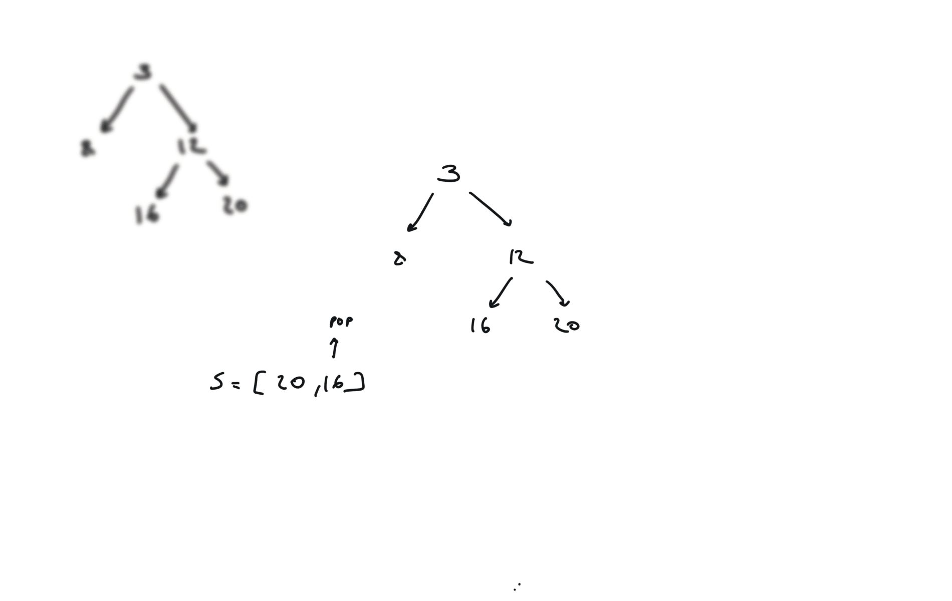
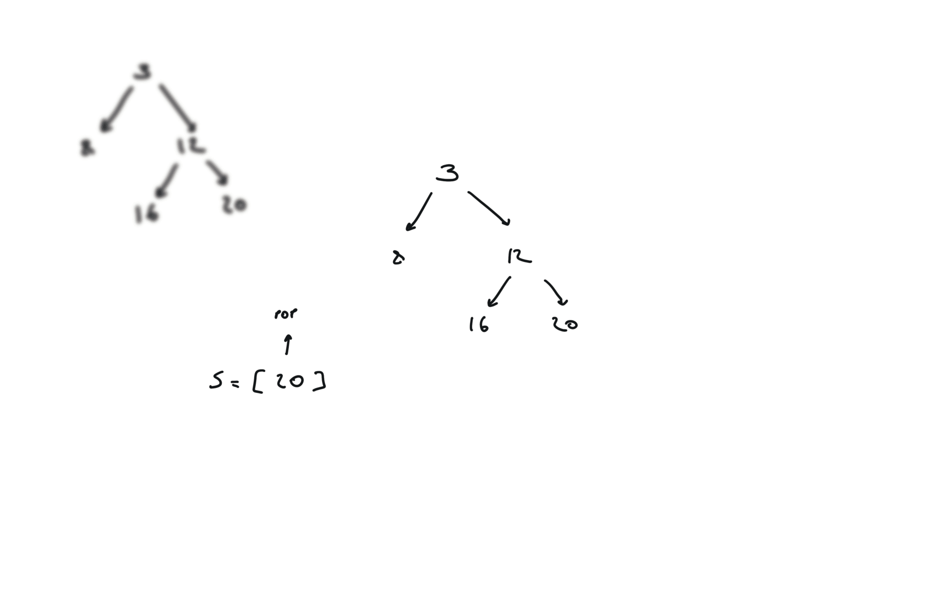
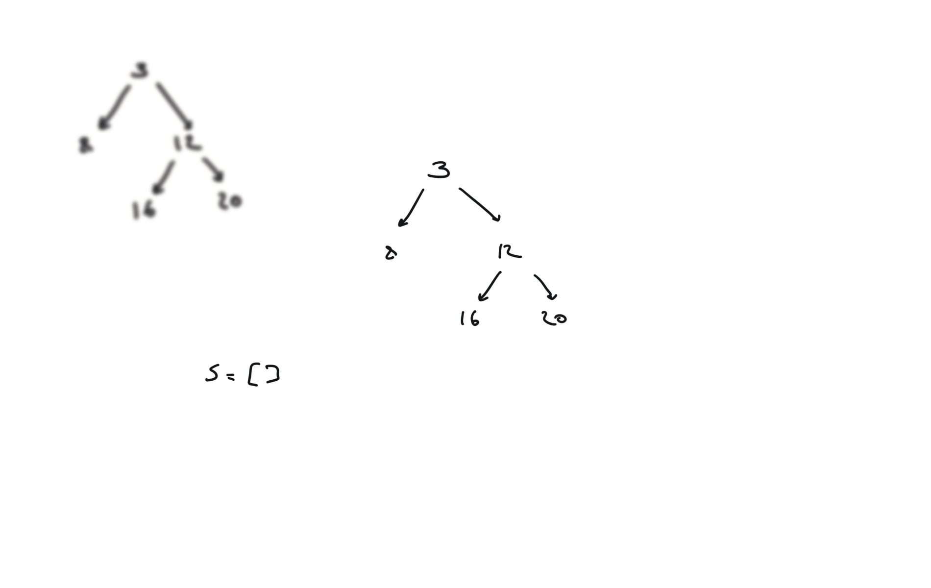
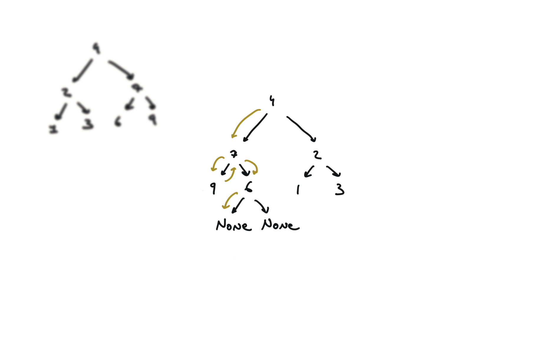
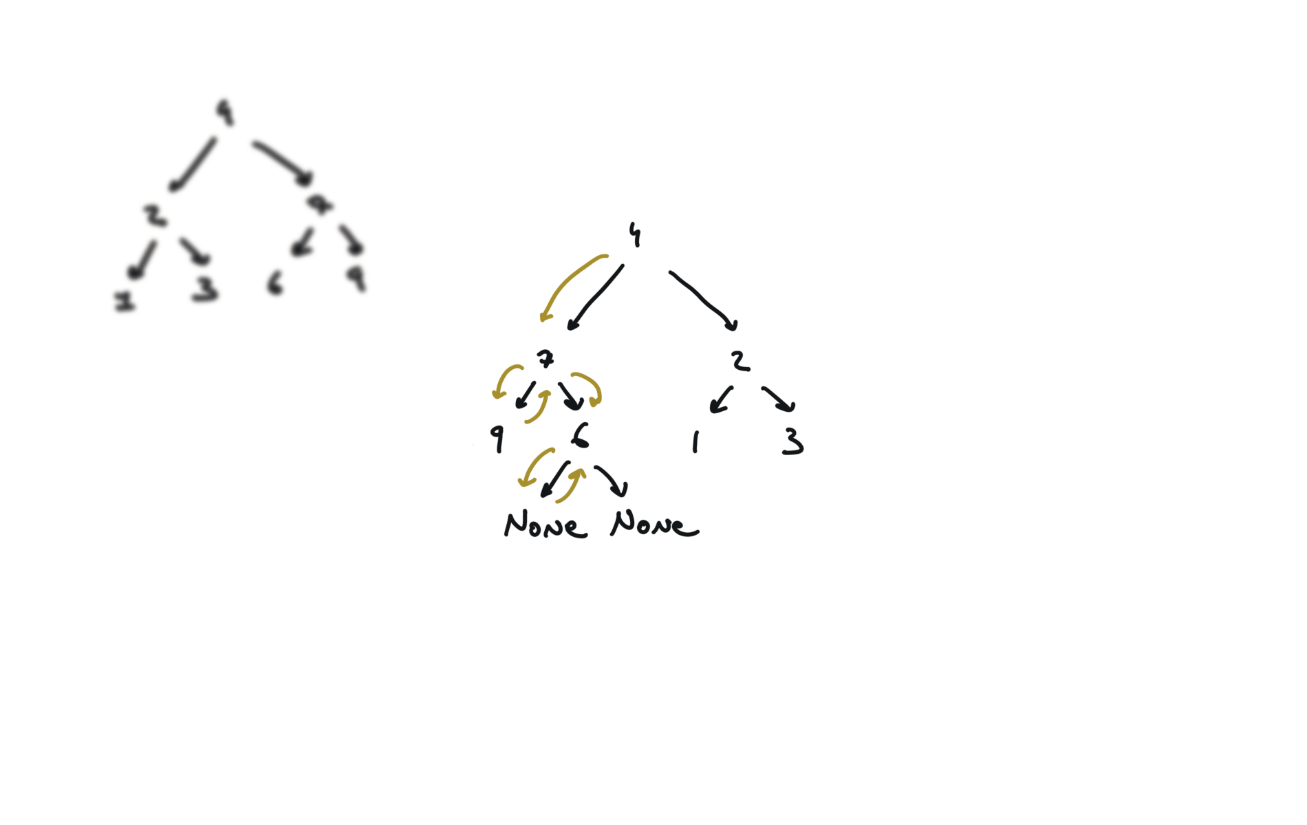
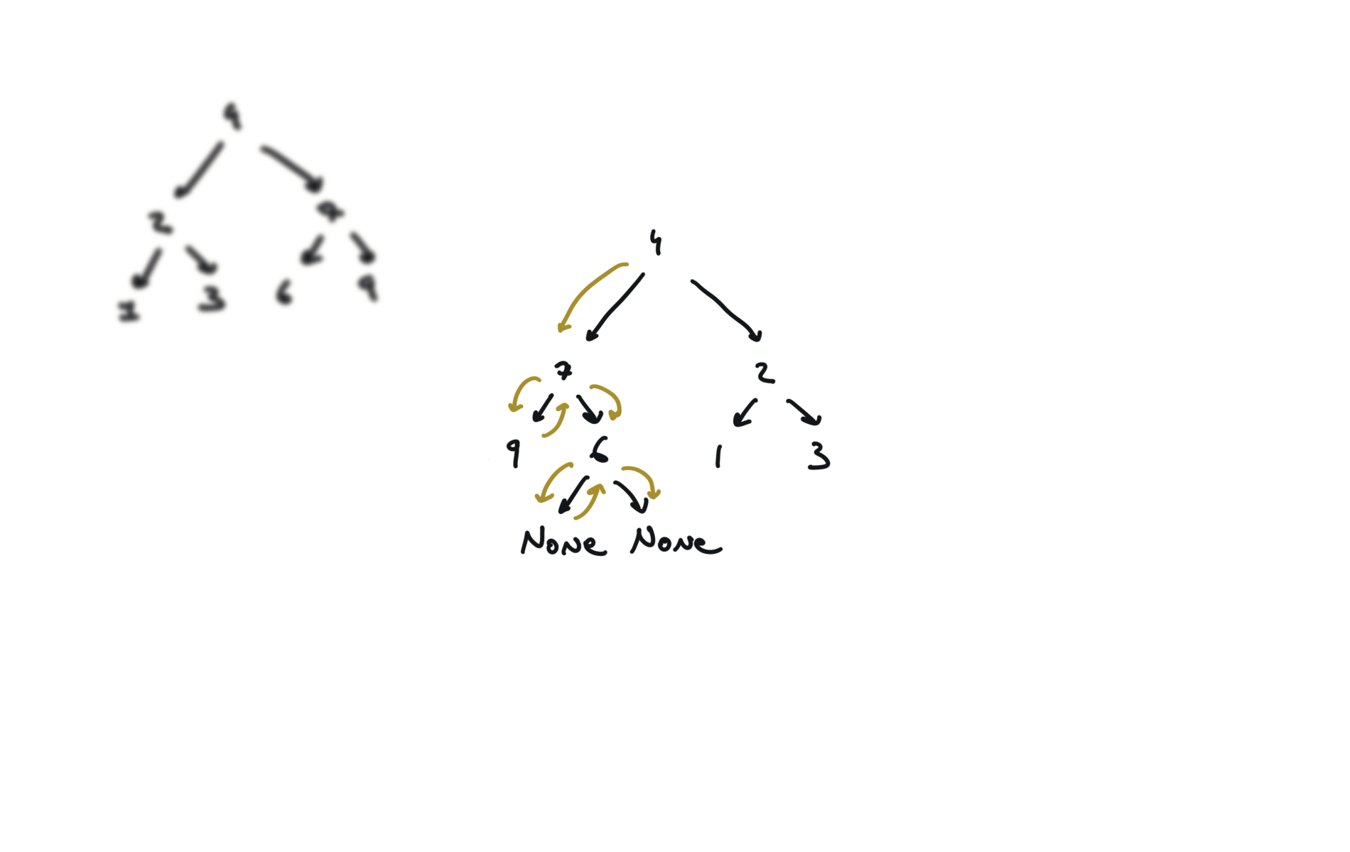
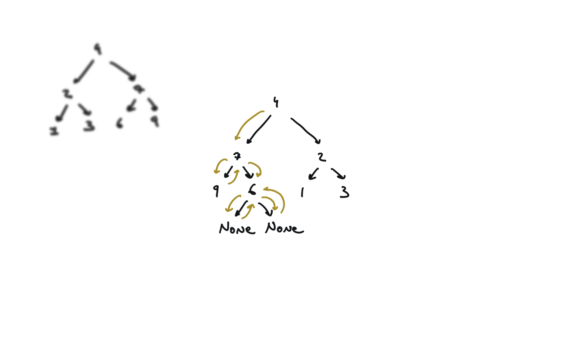
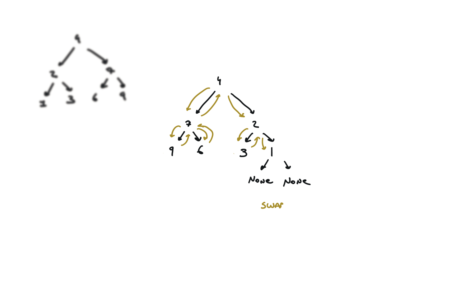
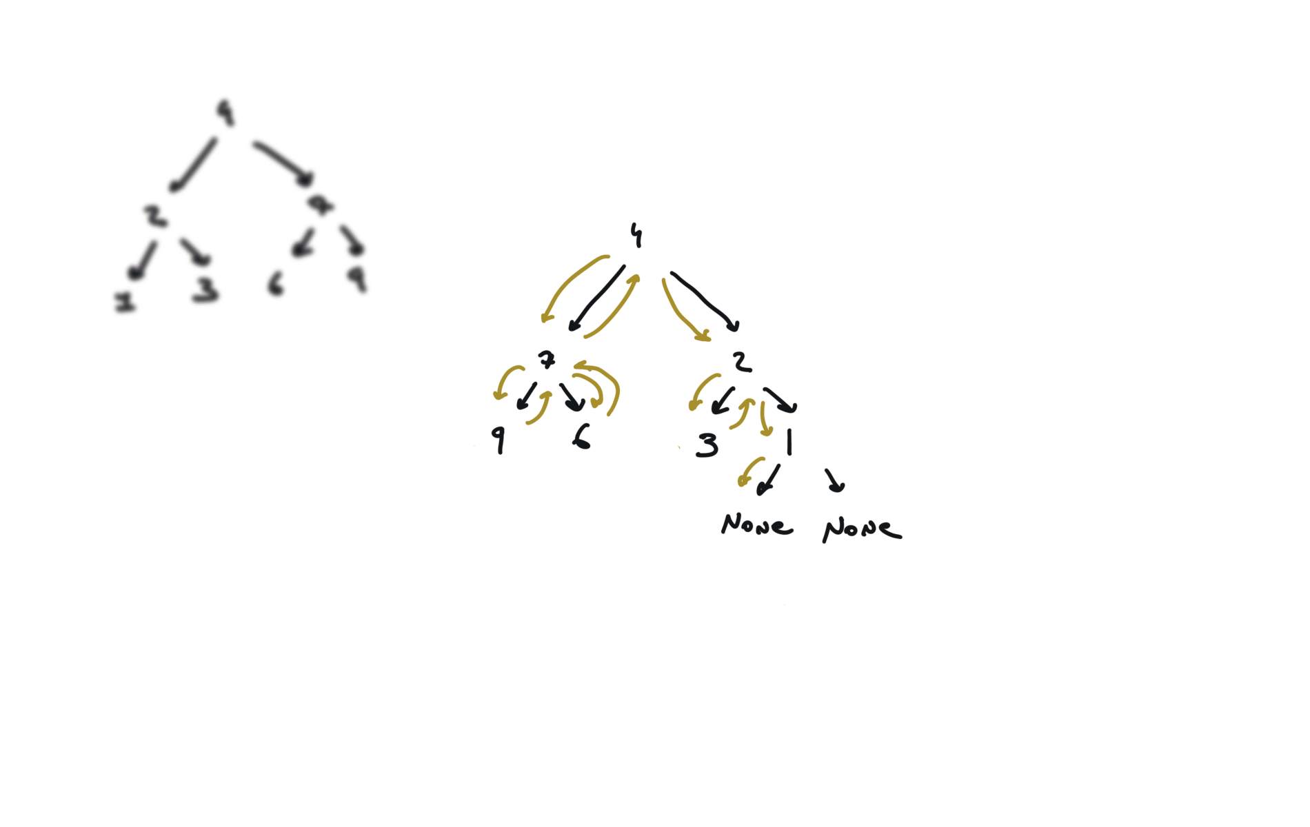
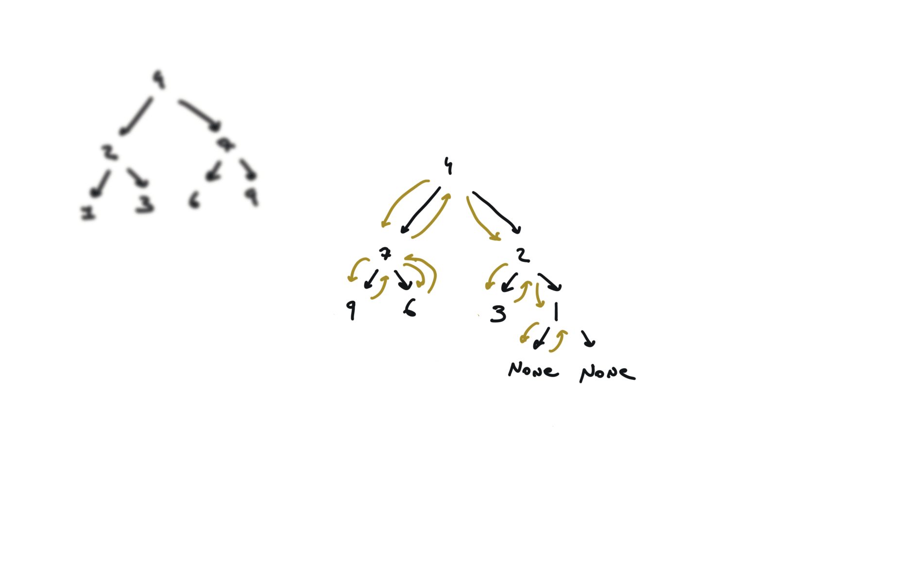
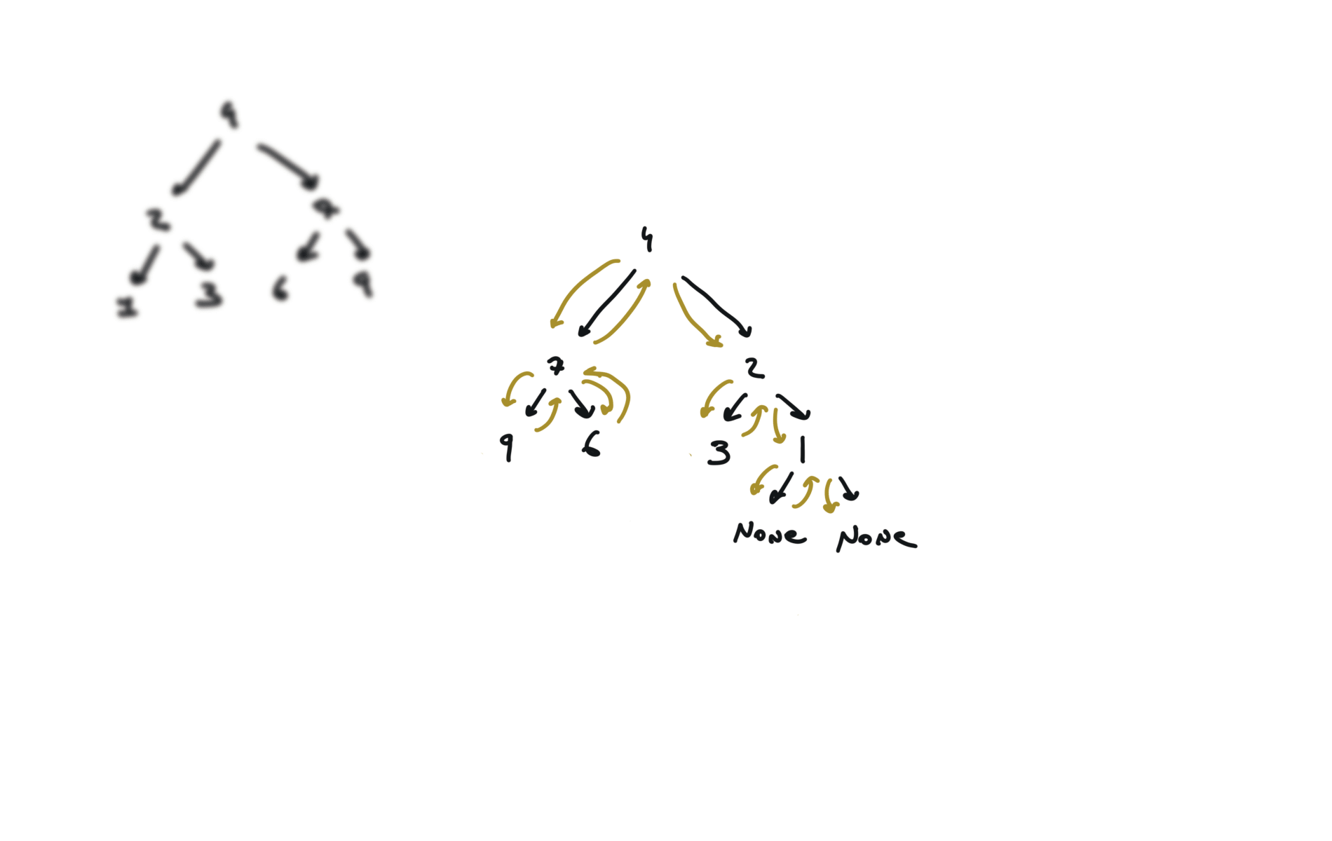
remember to put the right part first in the stack.
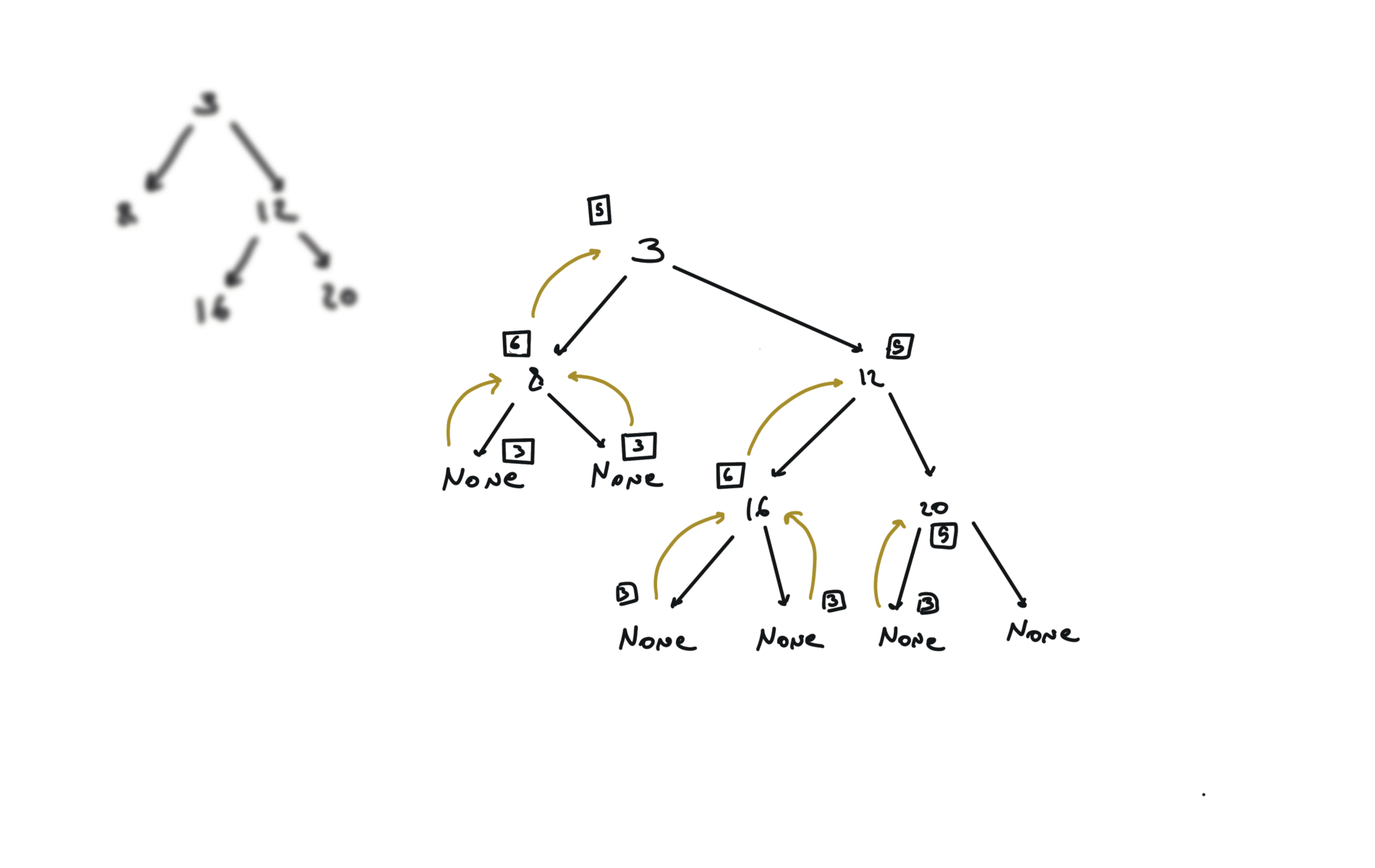
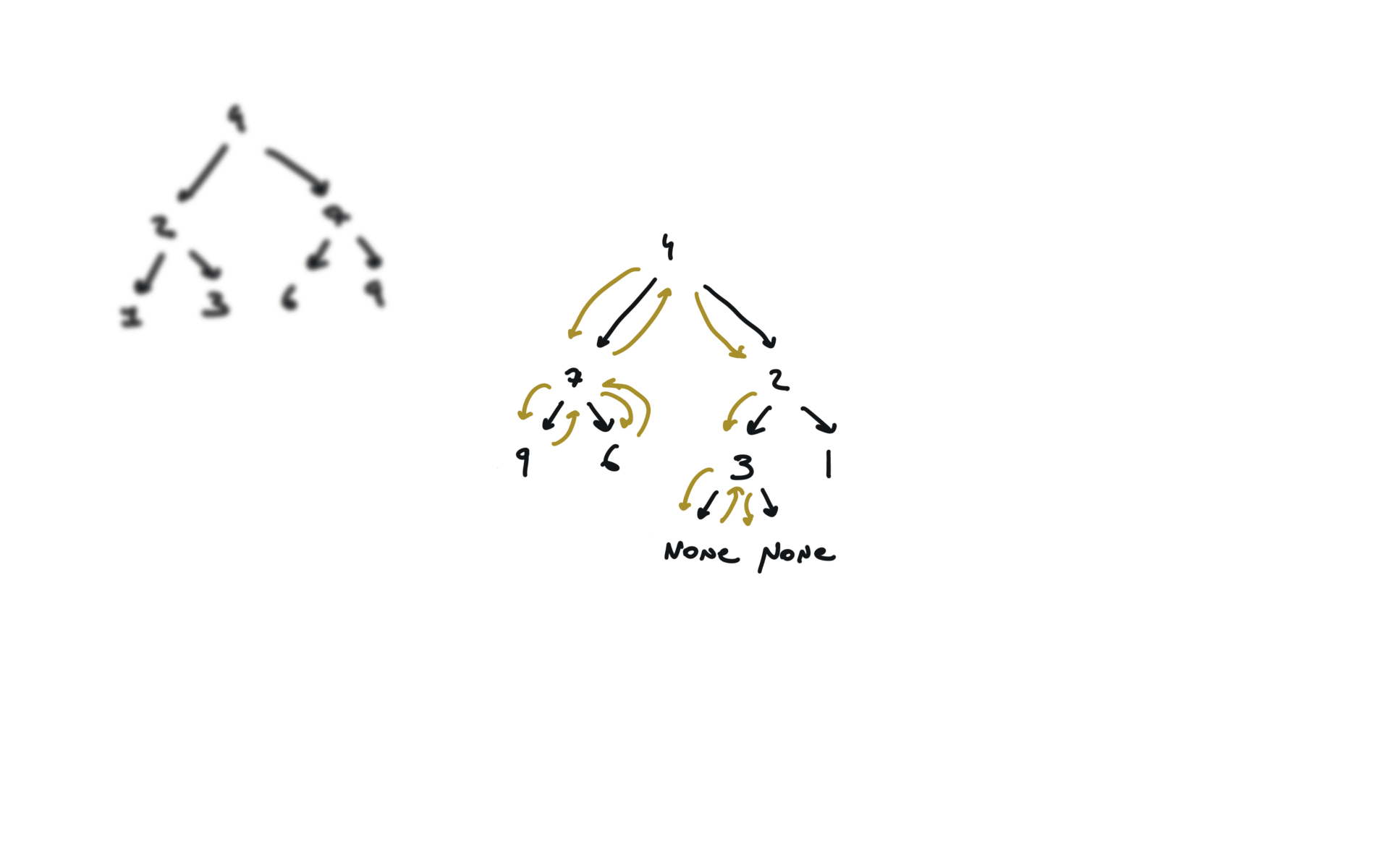
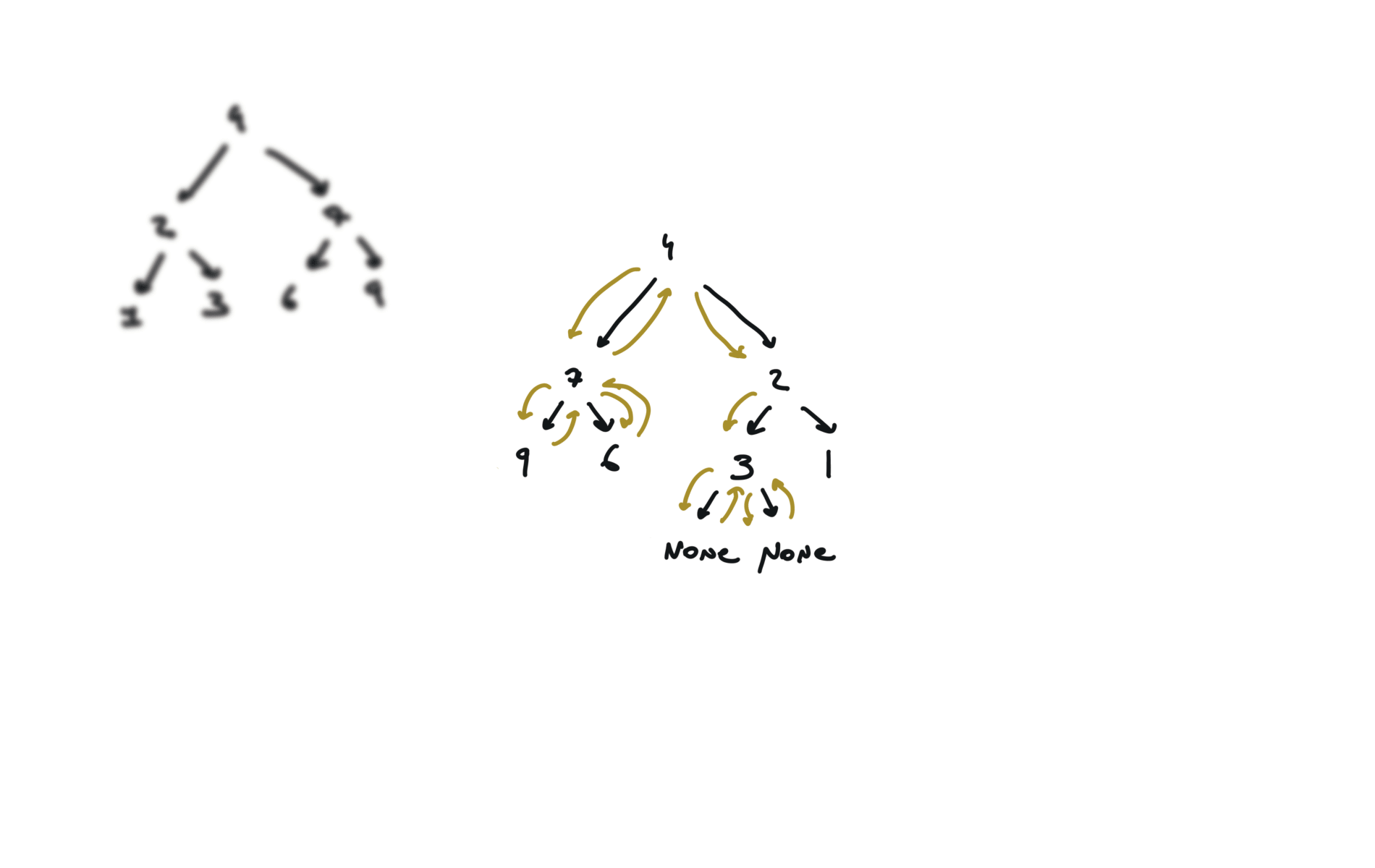
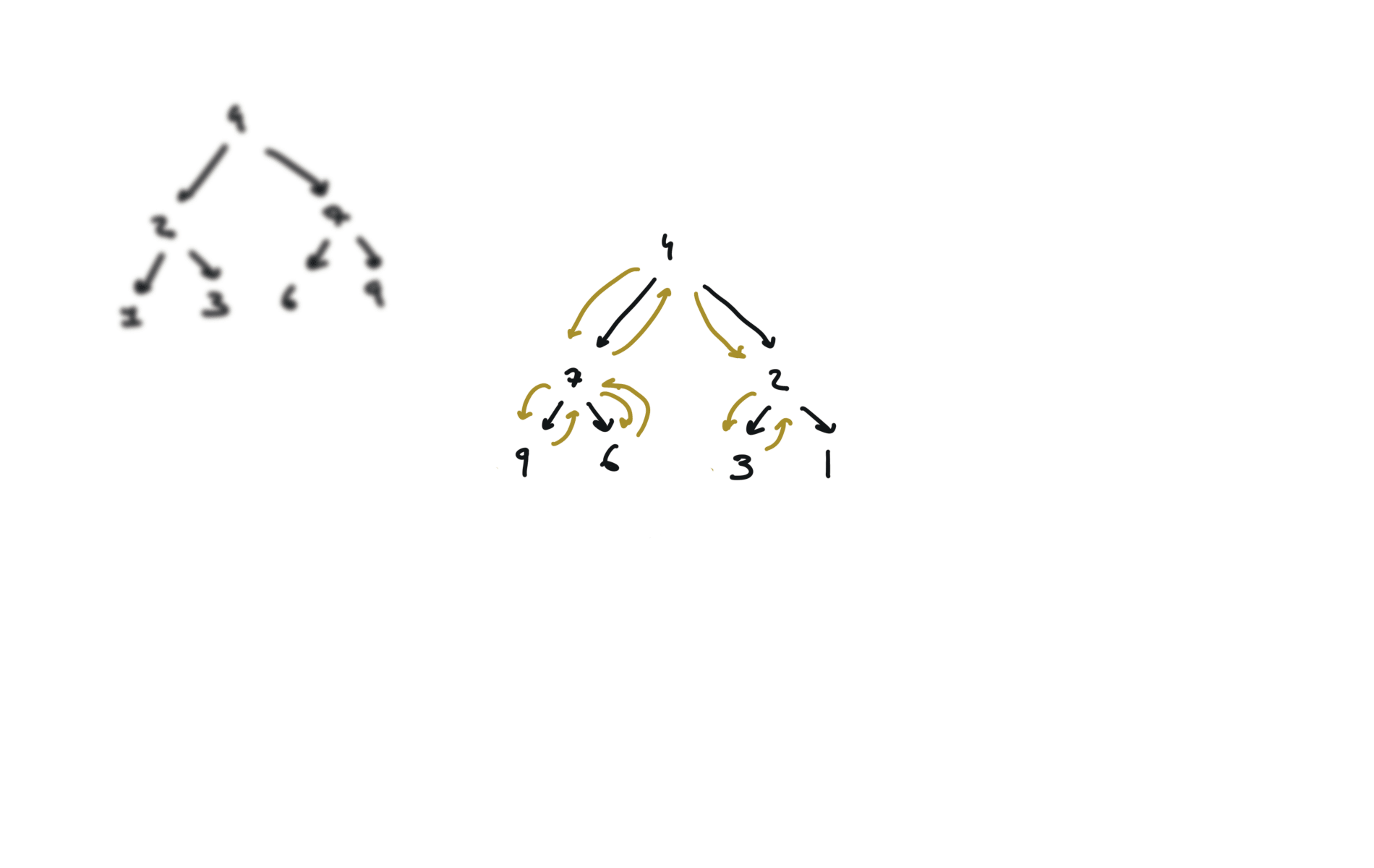
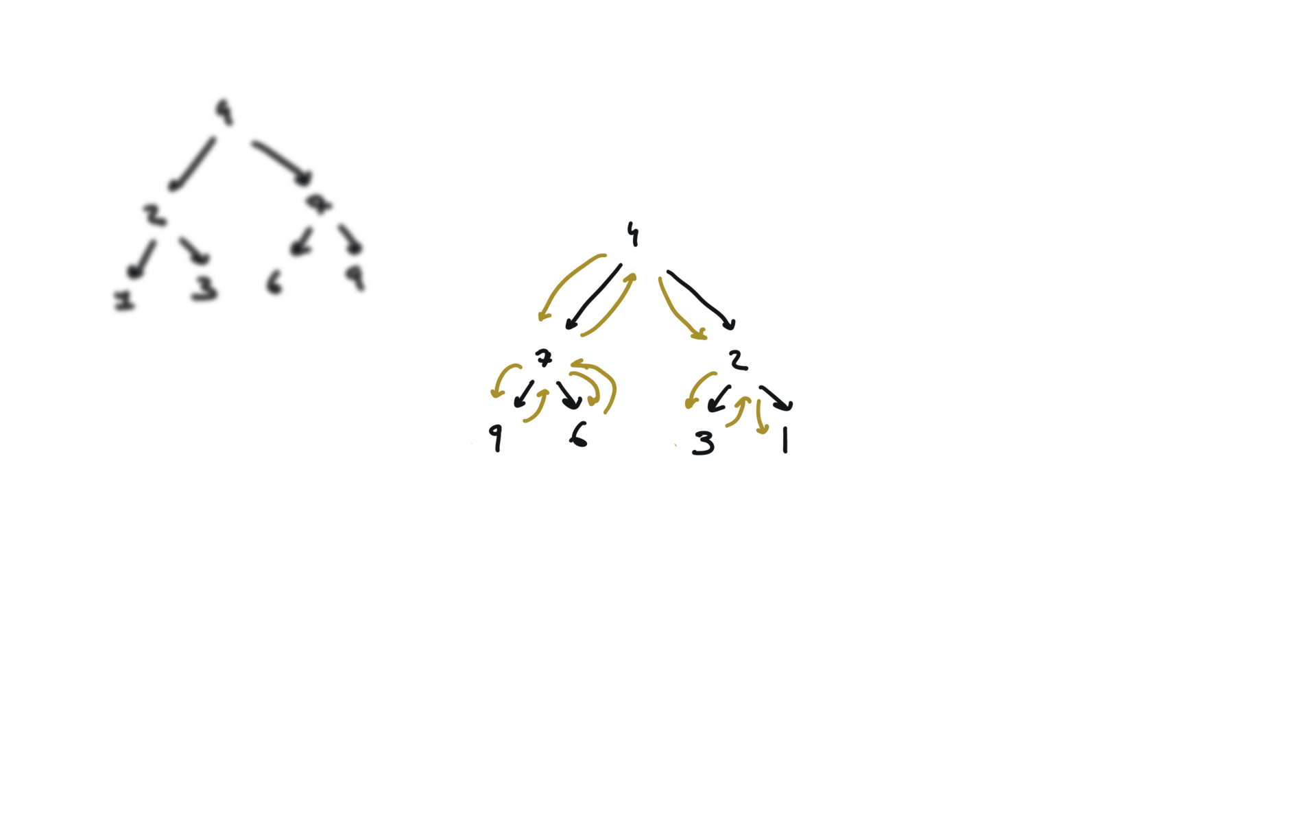
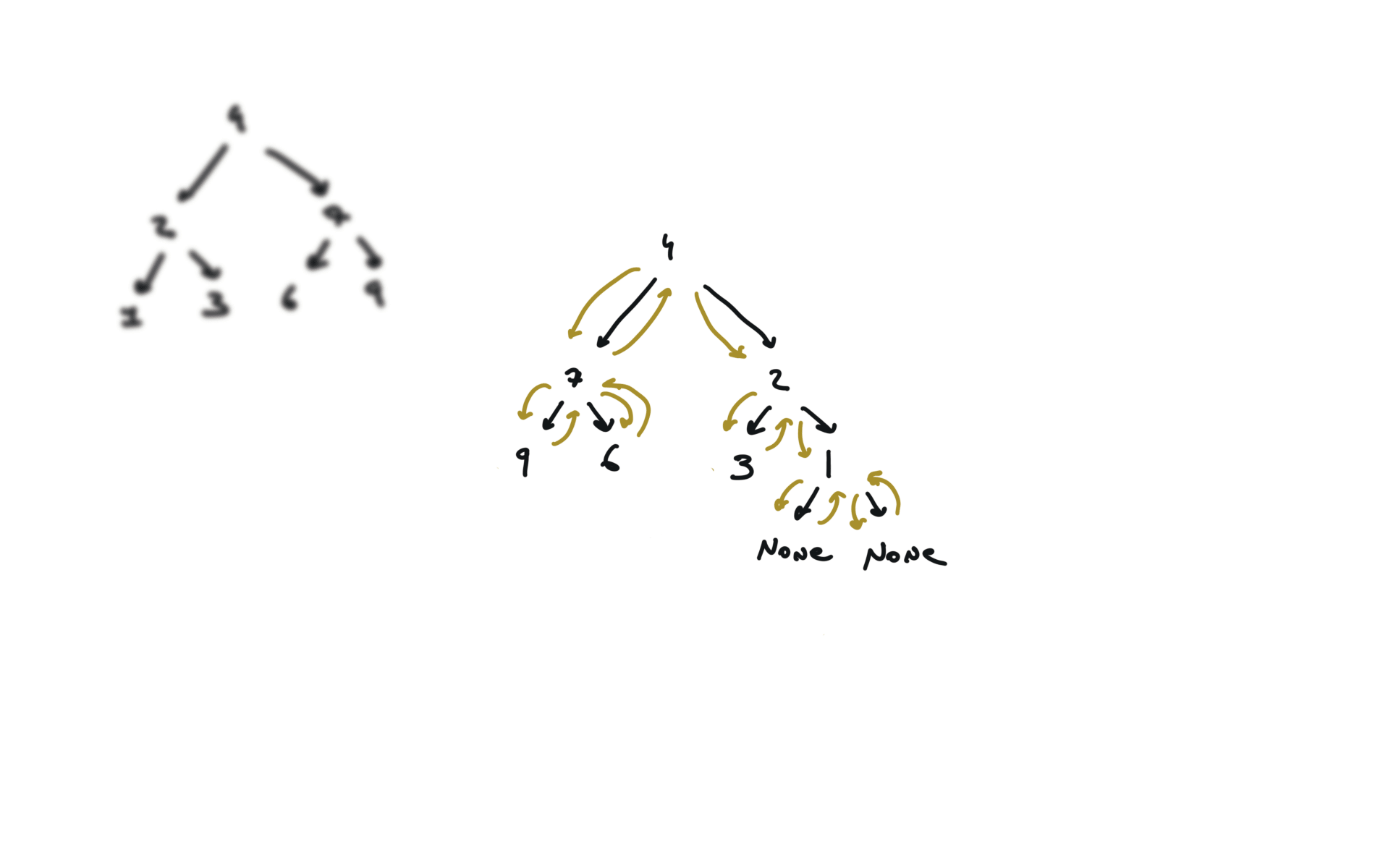
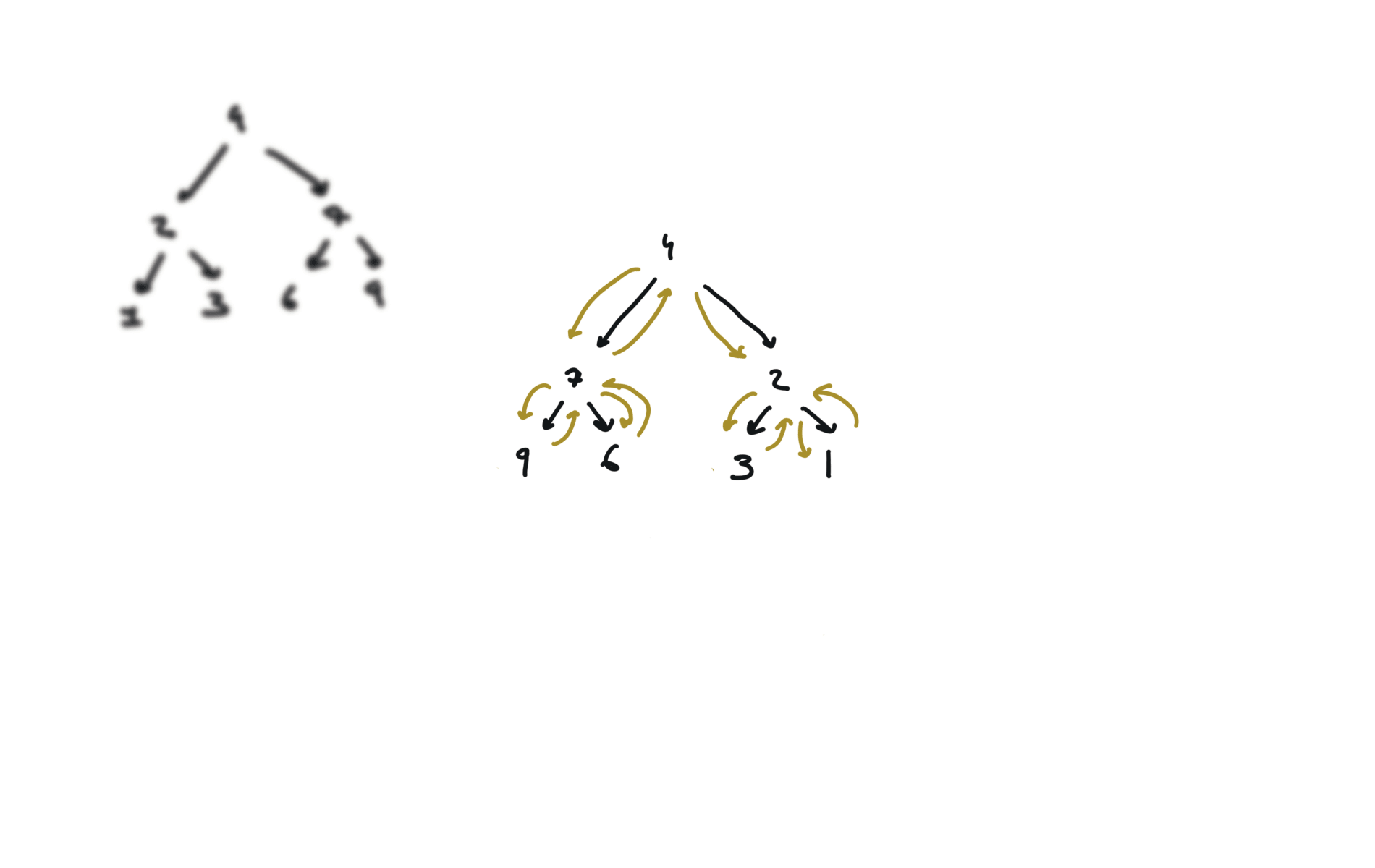
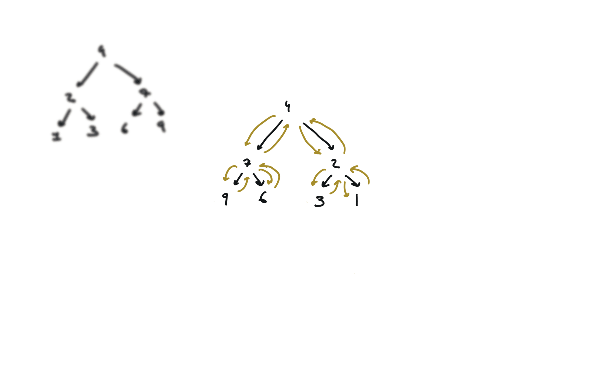
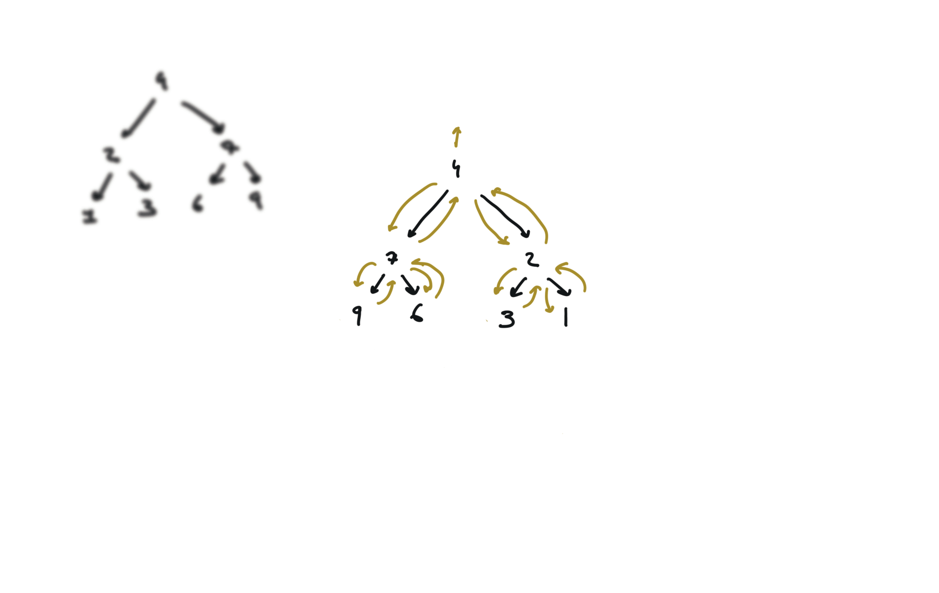
The time complexity of all visits is
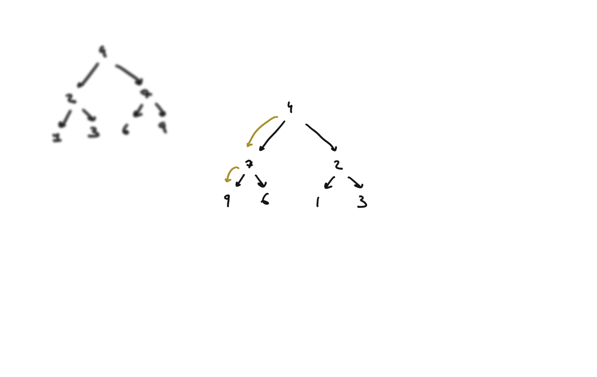
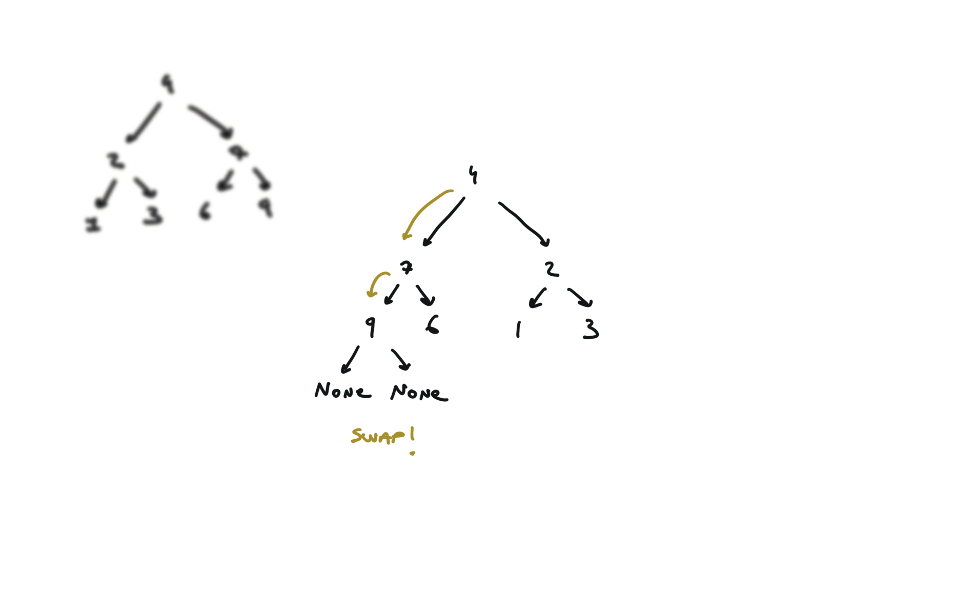
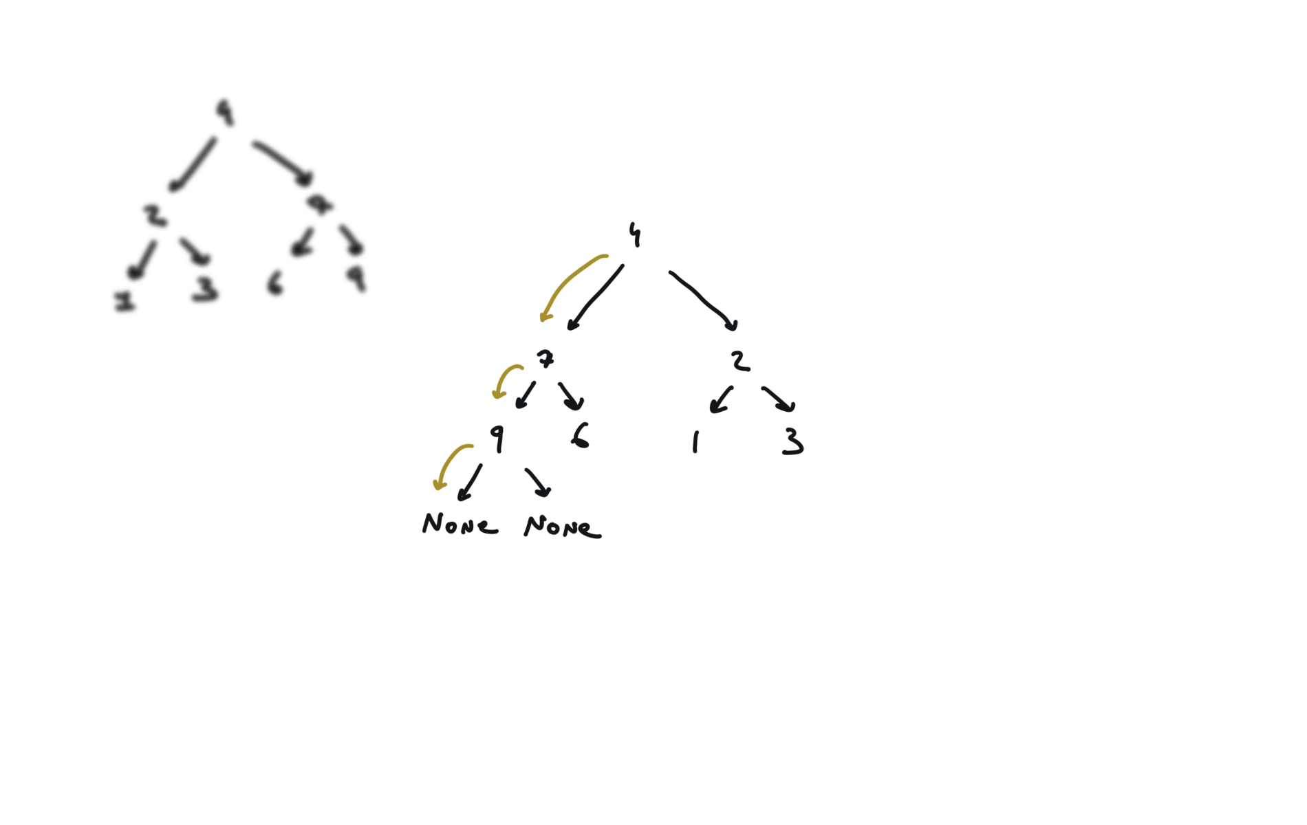
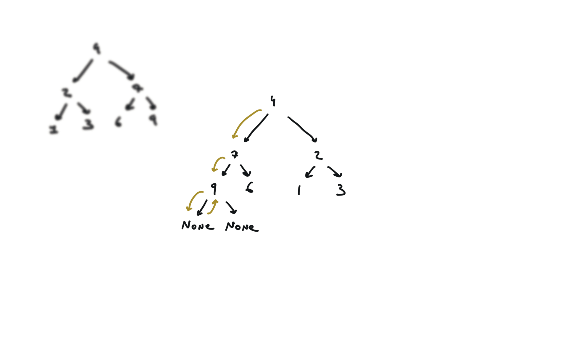
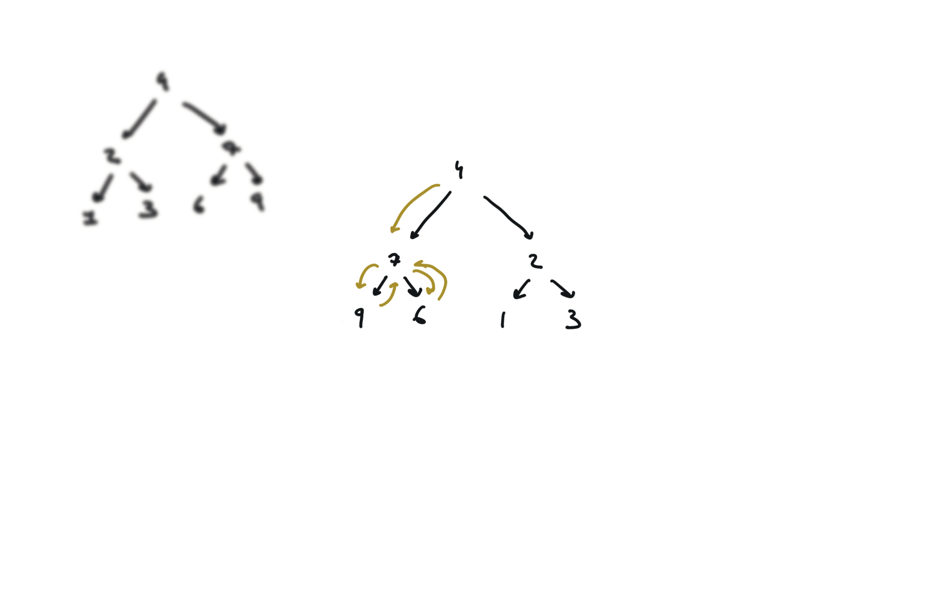
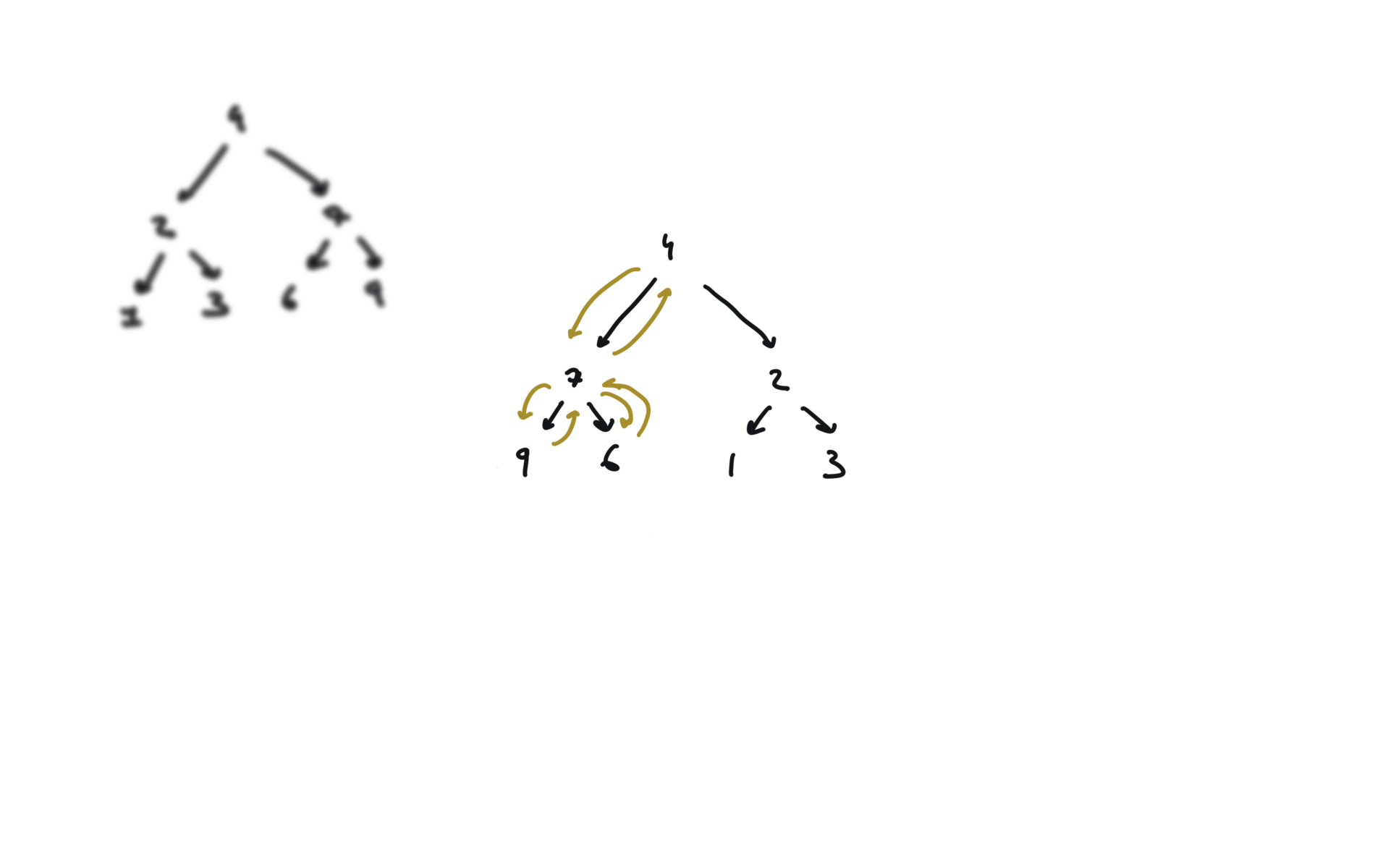
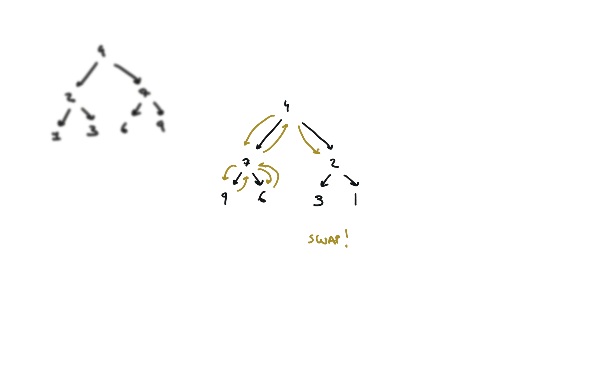
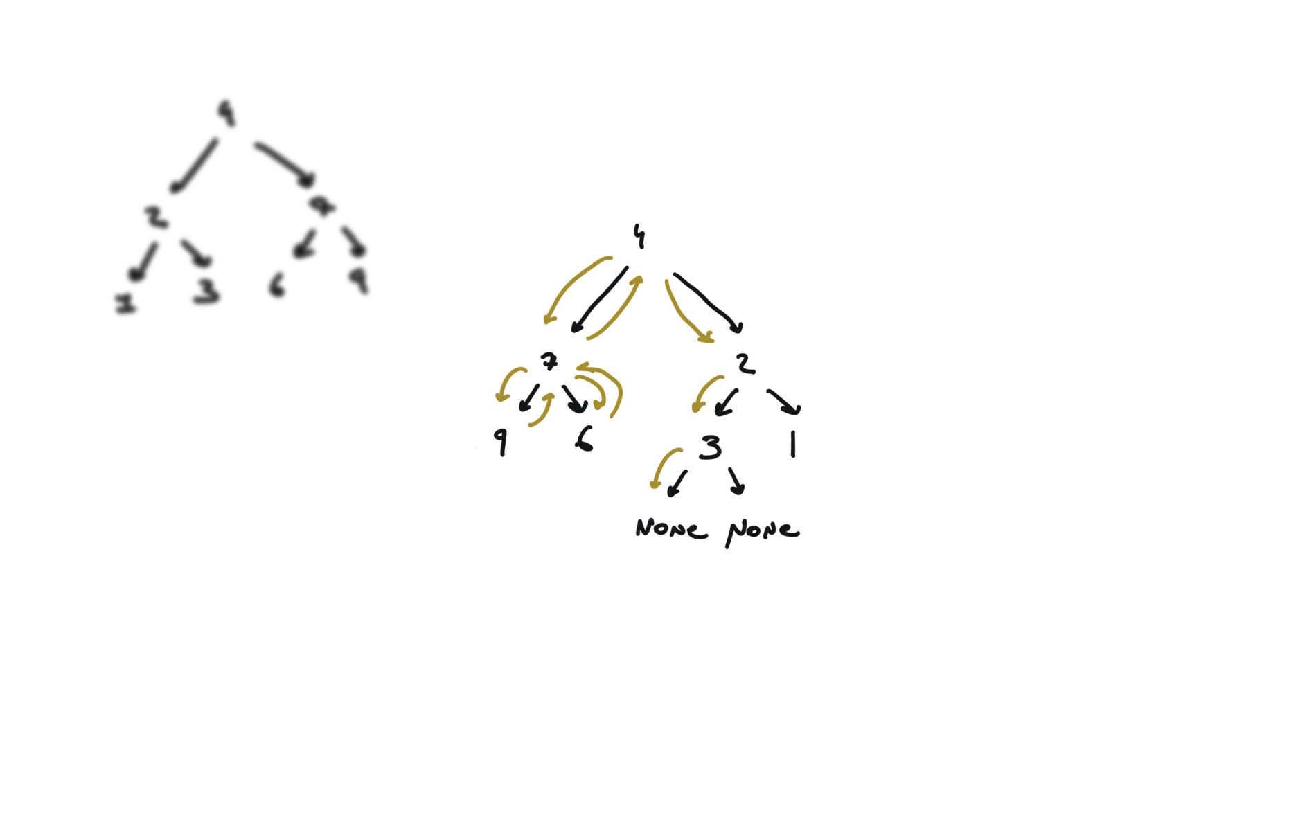
$$O(n)$$ Because we can write the complexity of the visit like this $$T(n) = T(k) + T(n-k-1) + 1$$ where k is the number of nodes on one side of the root and n-k-1 on the other side.
Let’s take in account 2 cases: The space complexity is the maximum length of the recursion stack (recursive) or the maximum length of the queue, which is $n$. $$S(n) = O(n)$$
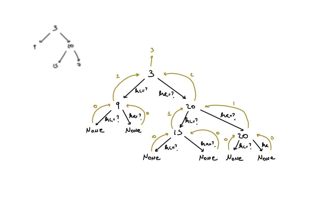
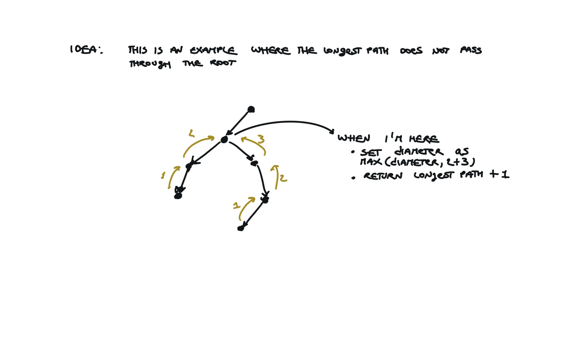
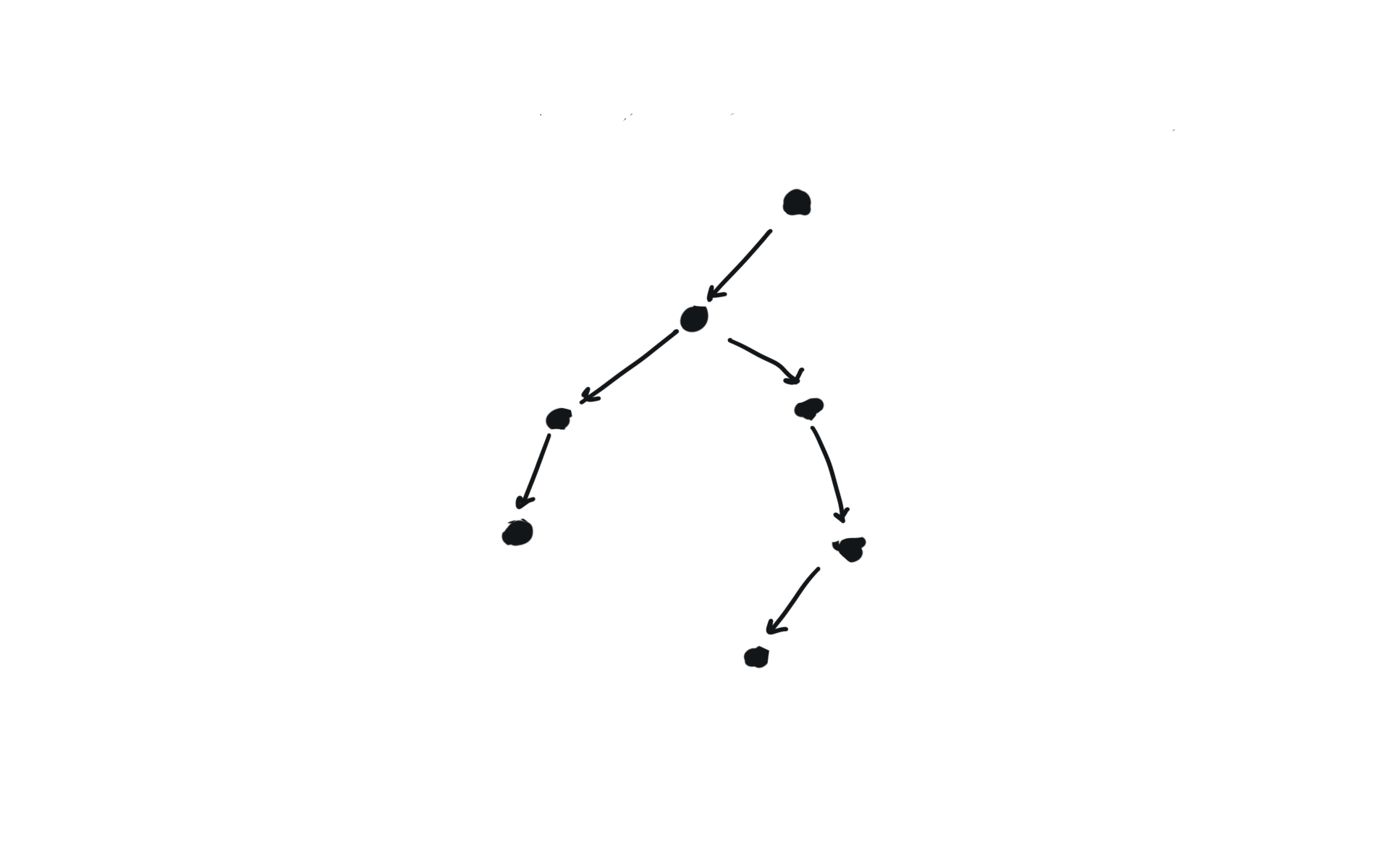
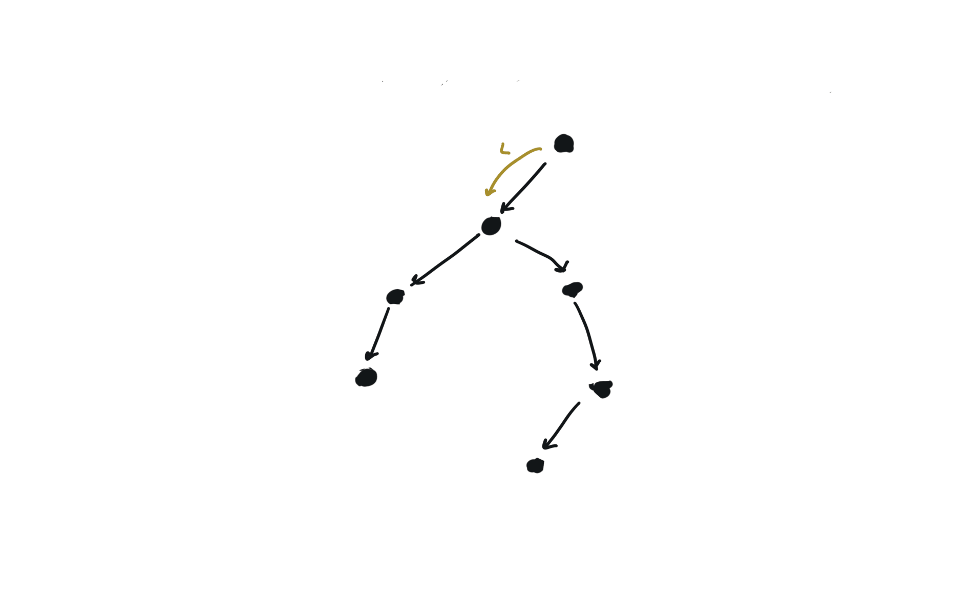
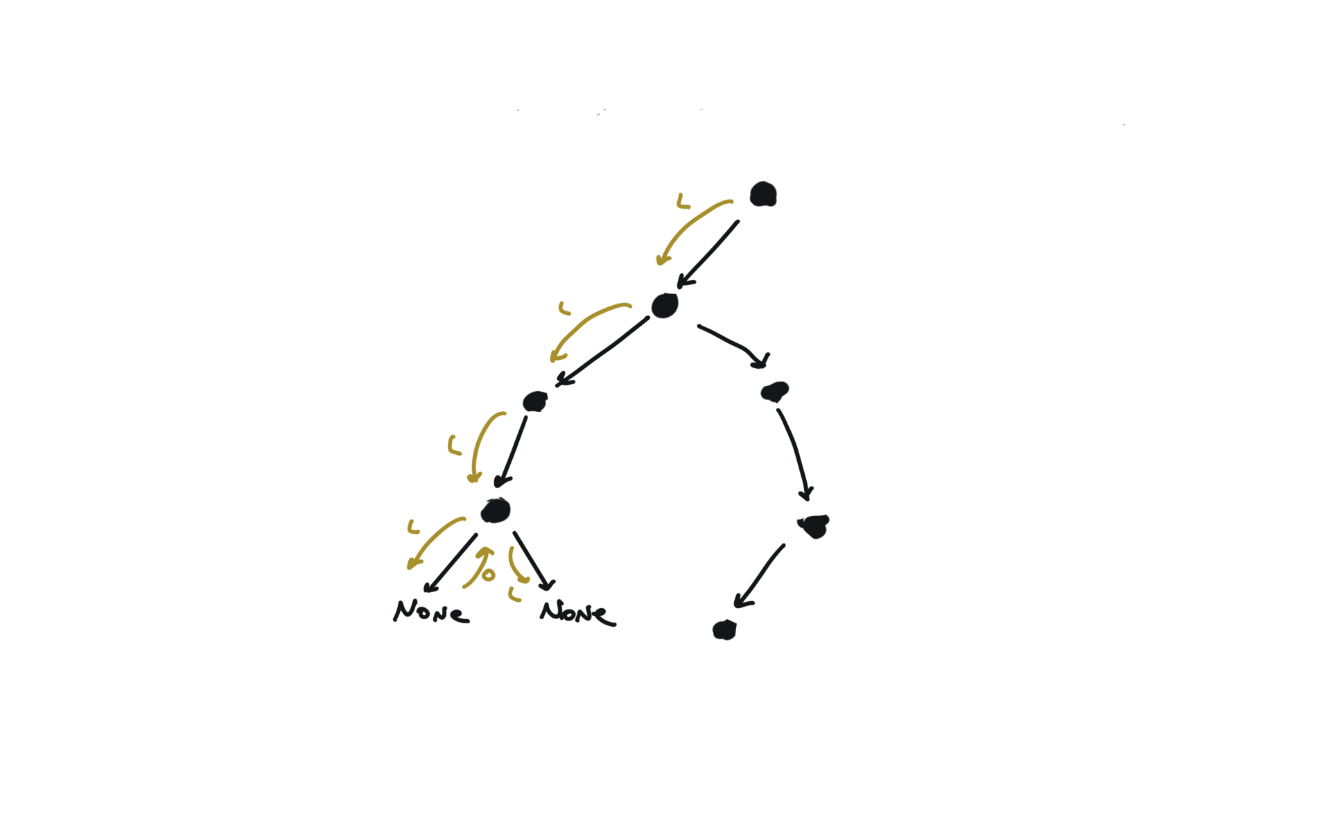
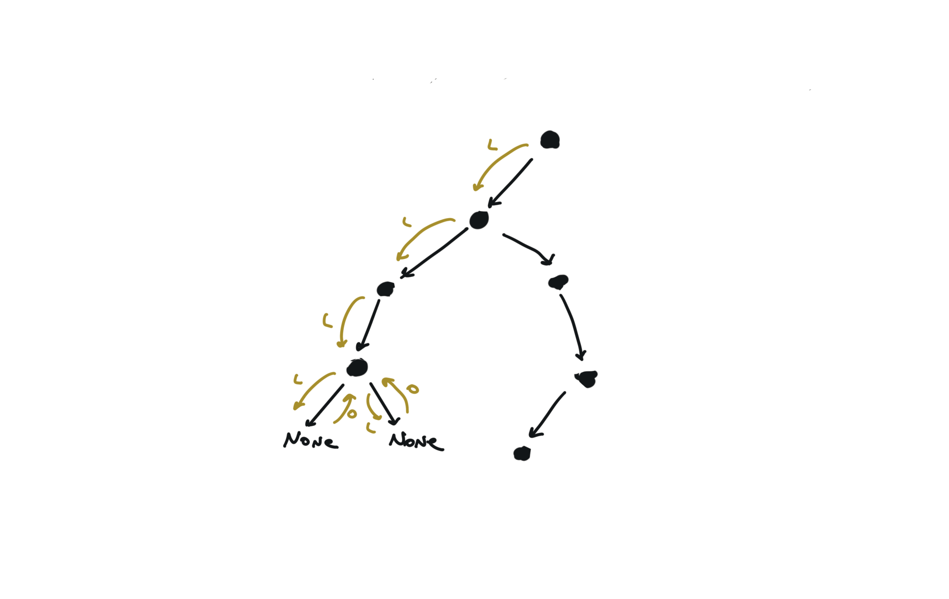
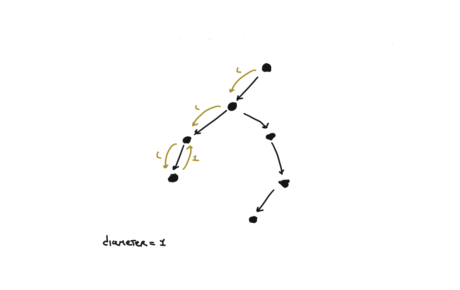
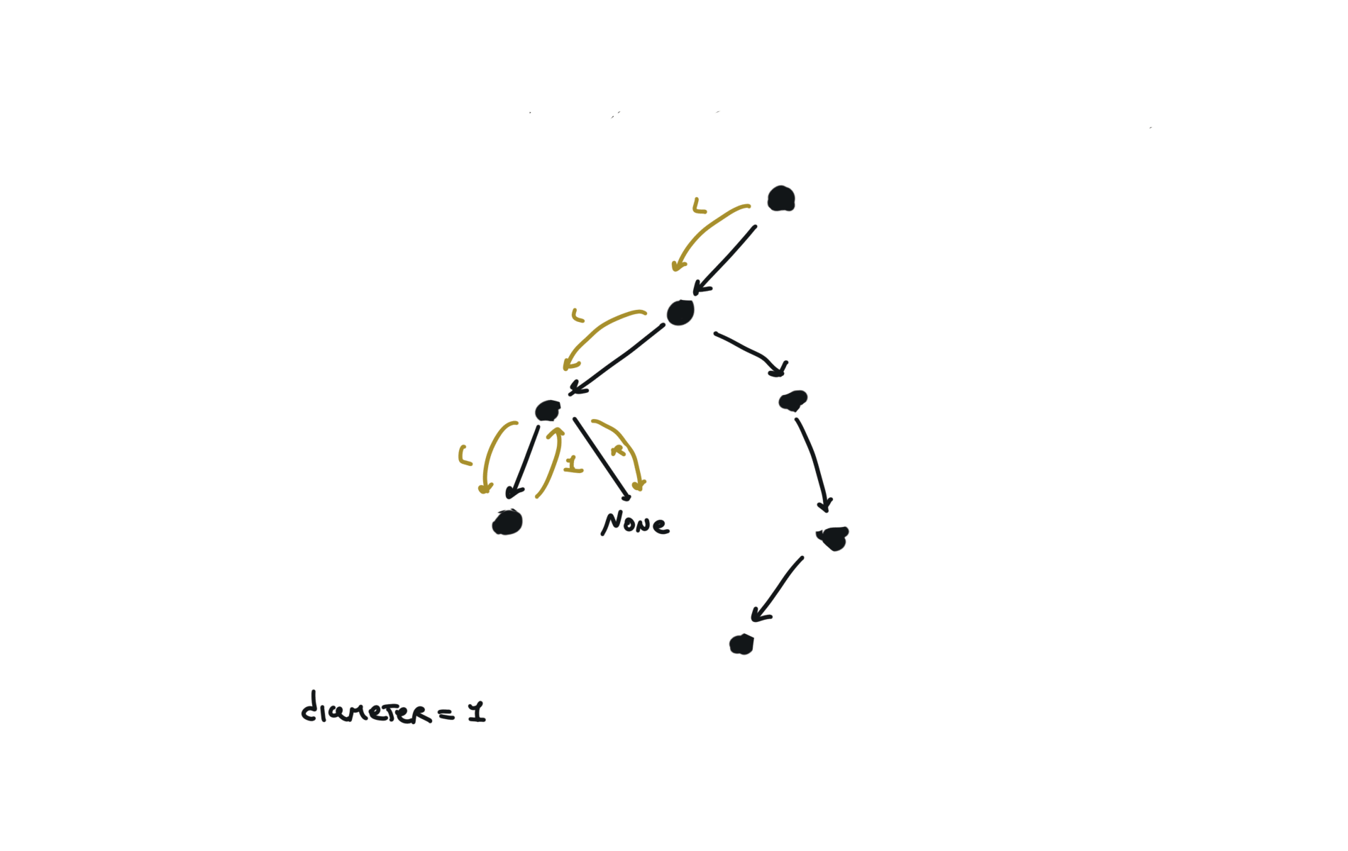
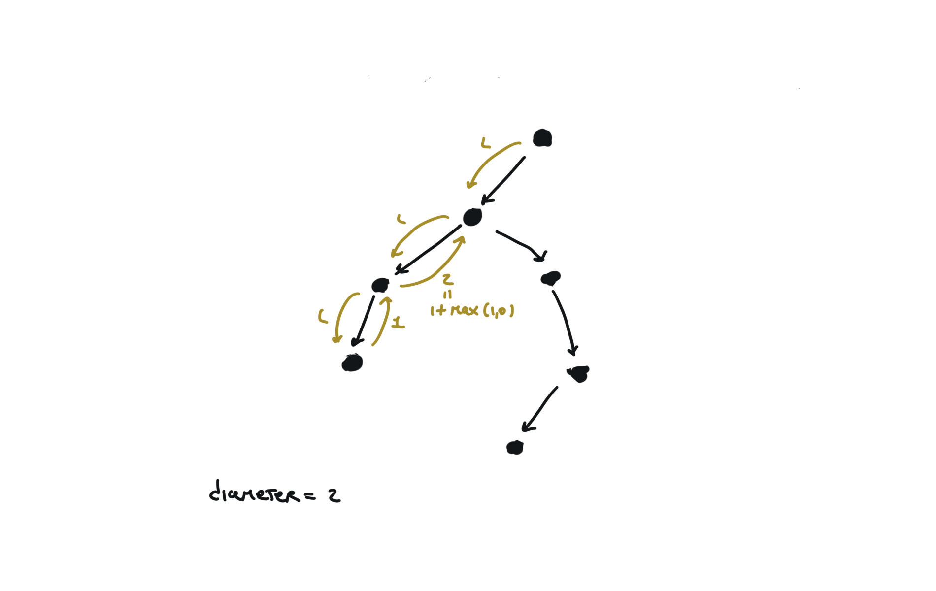
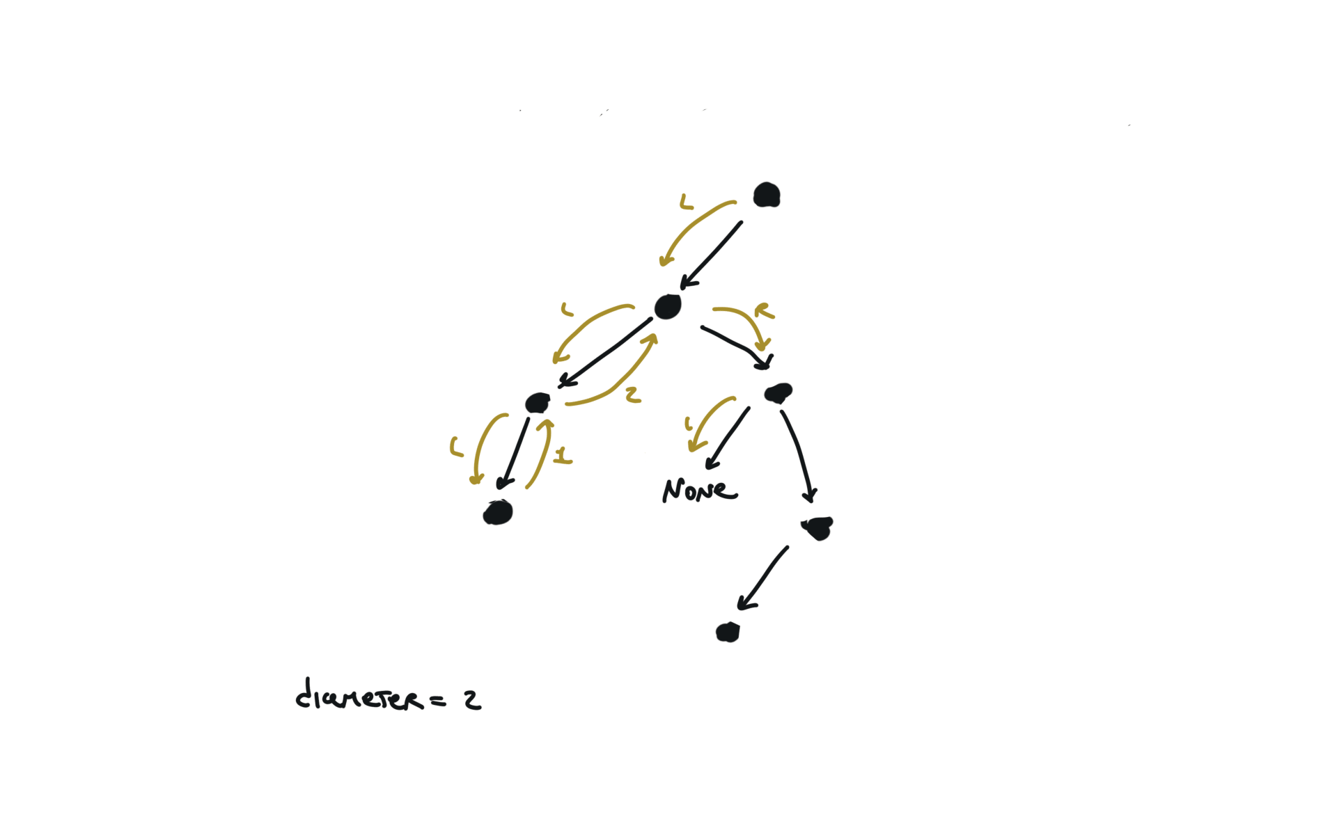
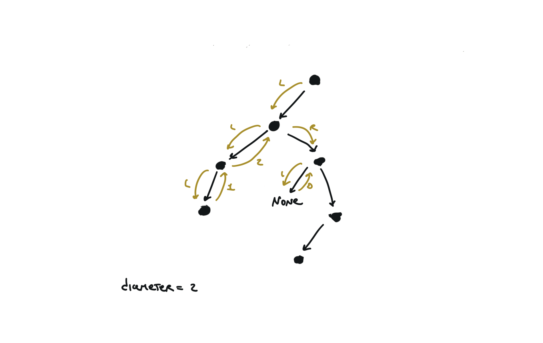
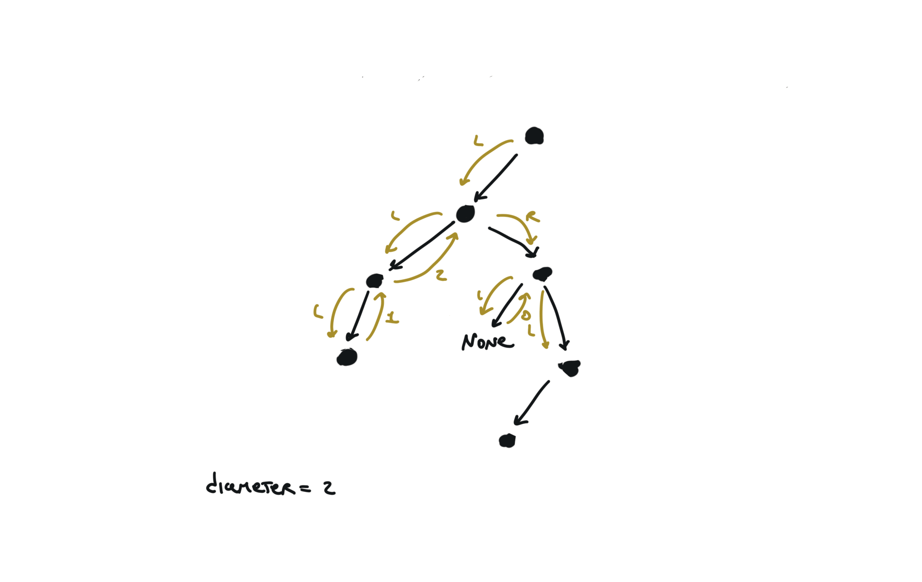
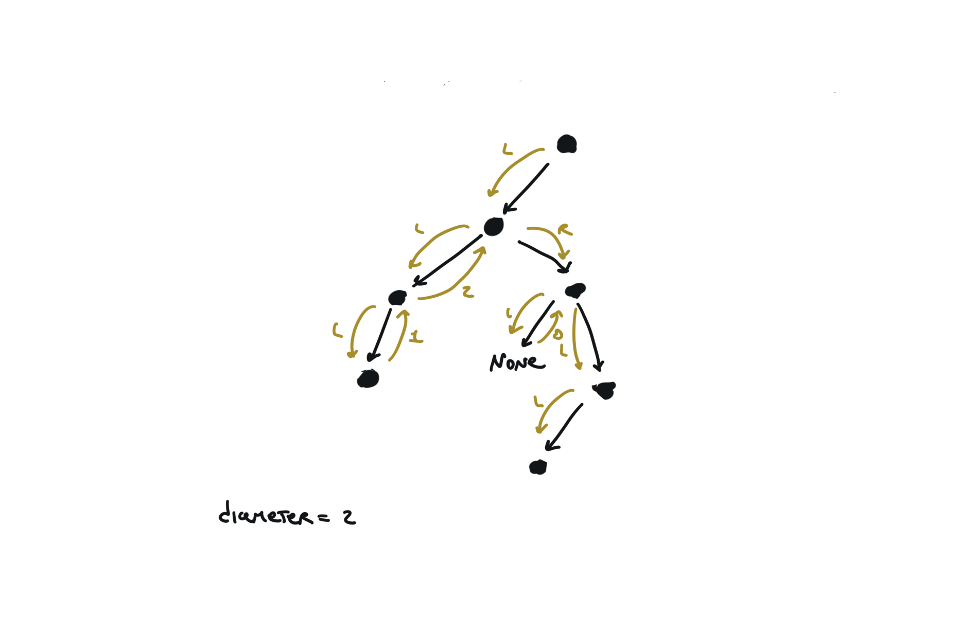
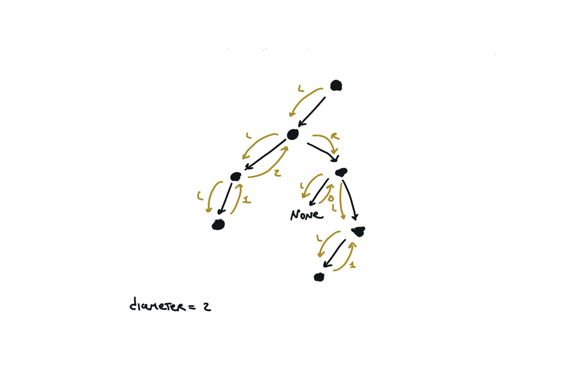
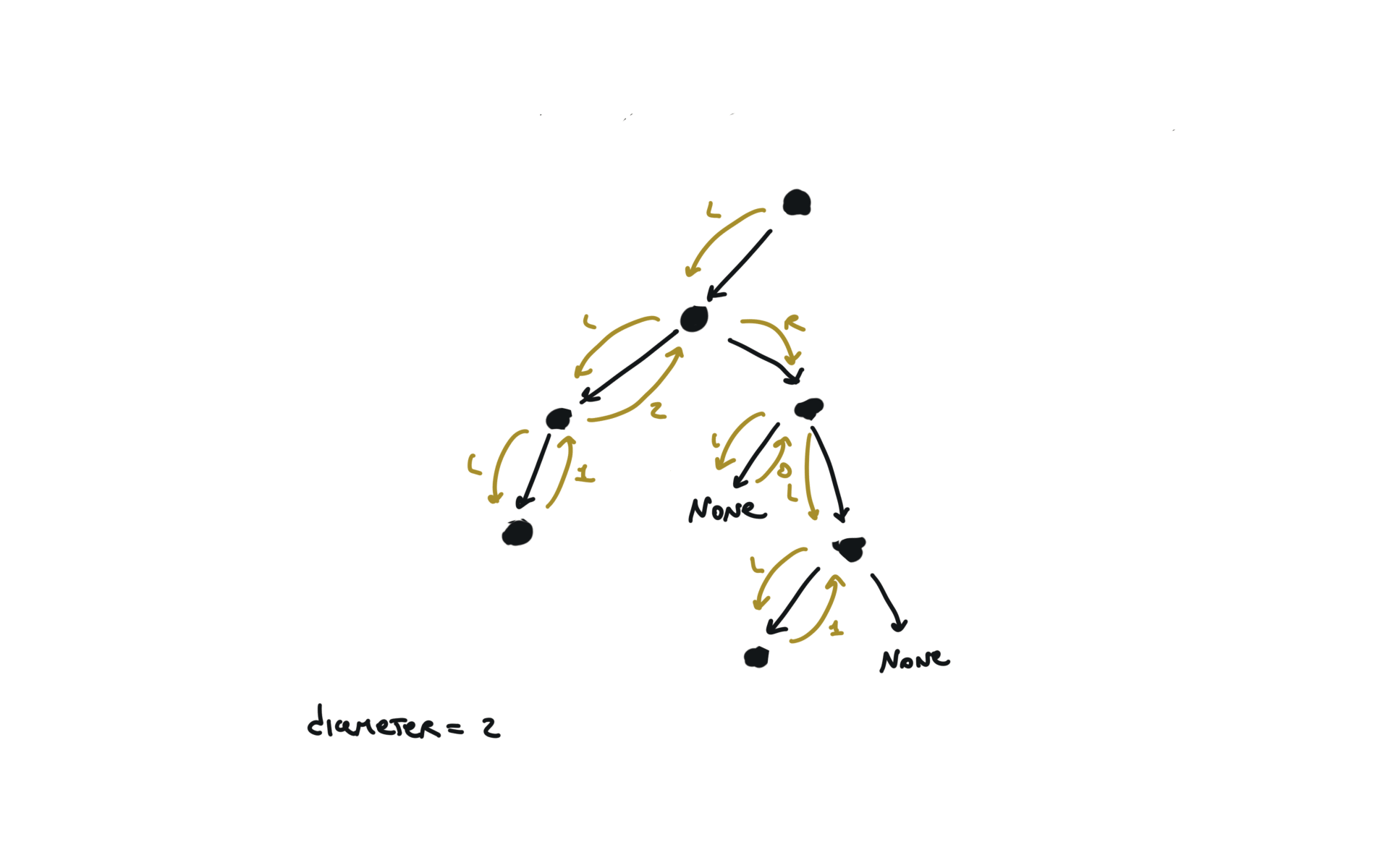
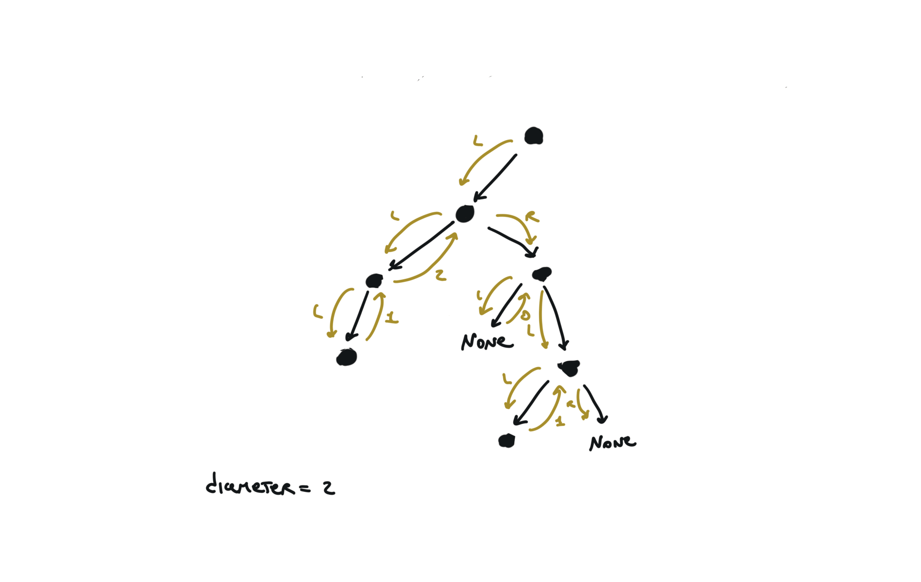
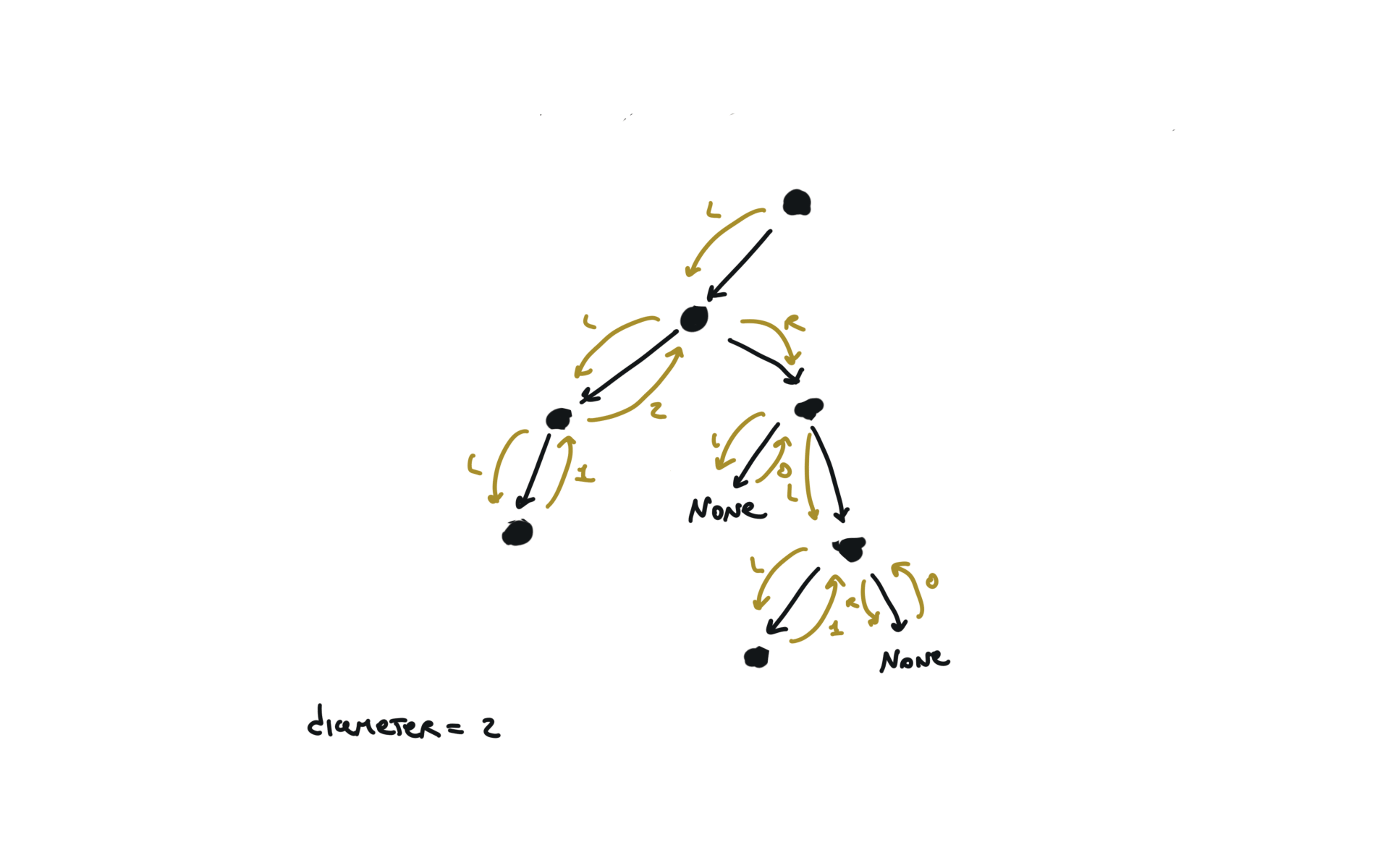
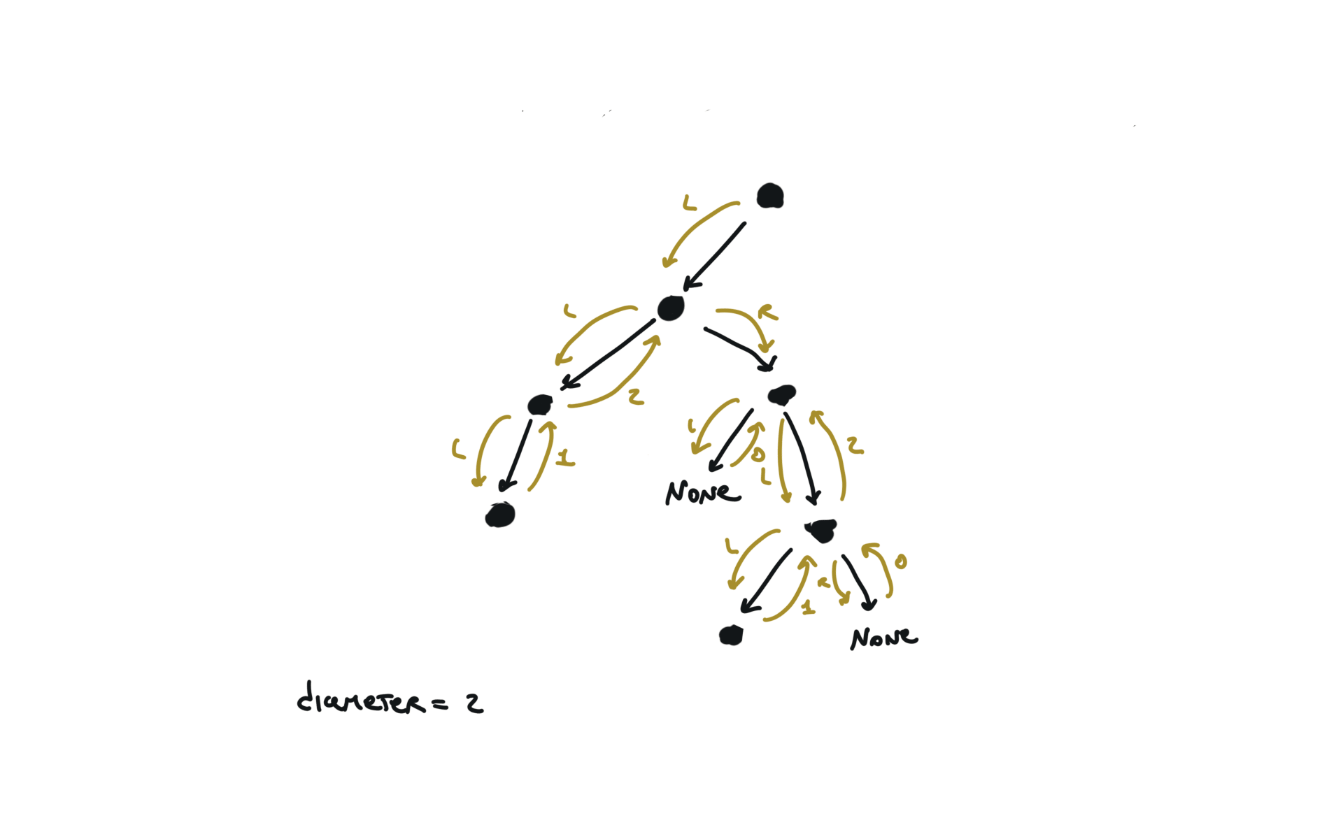
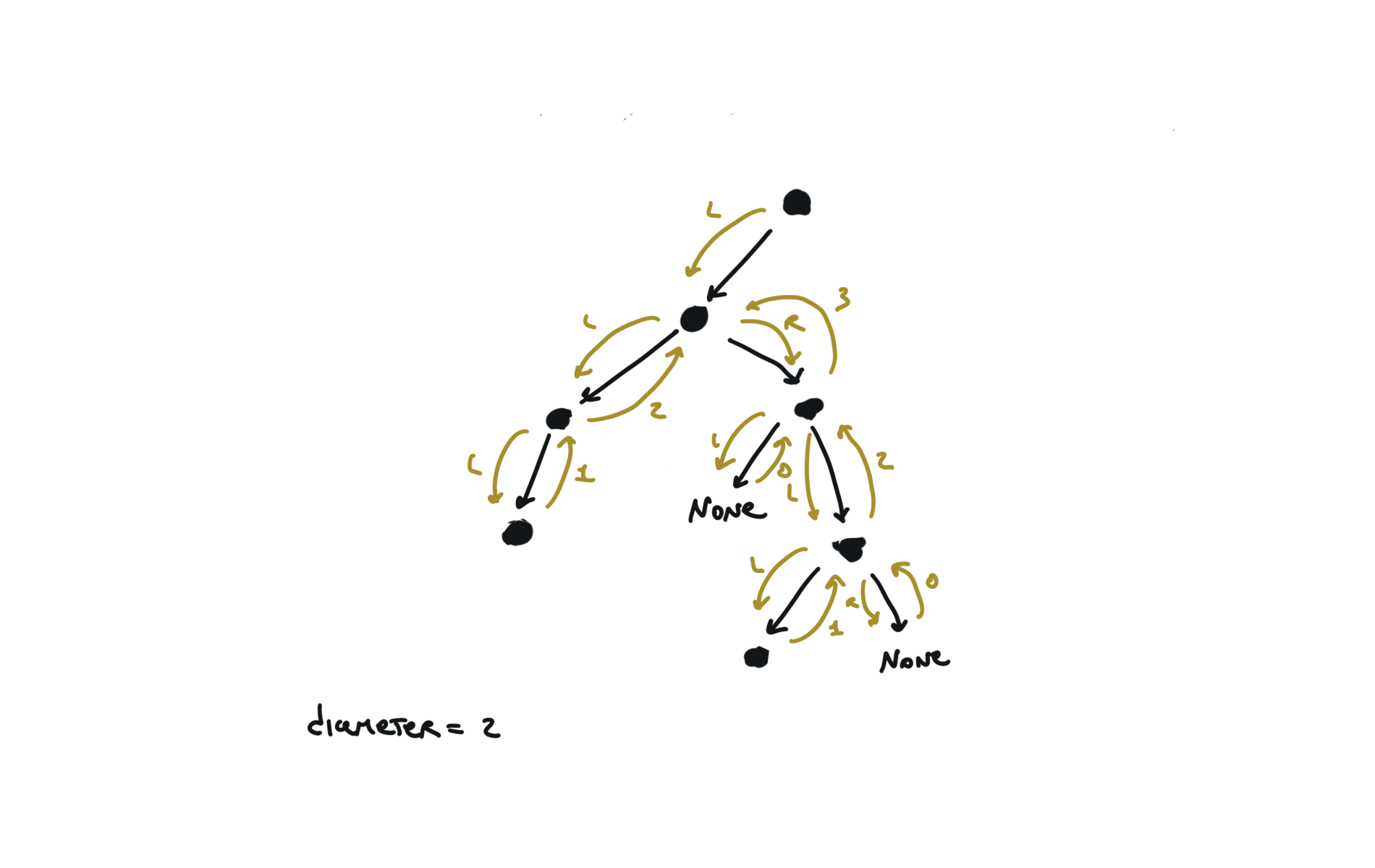
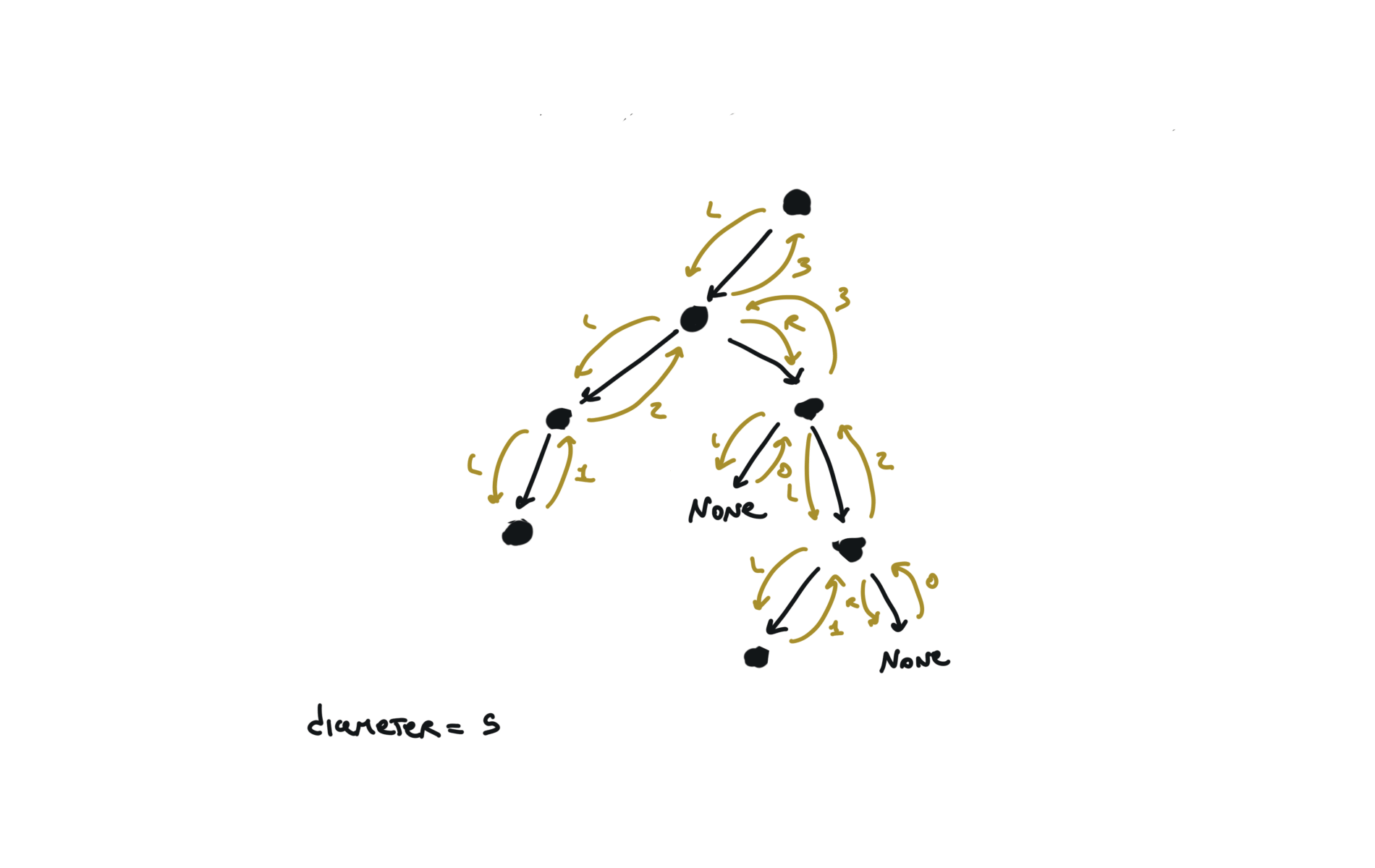
You can refactor this condition Which true/false table is the following: The condition becomes: The comparison with the value can be at the beginning. For each node, i check if it is the same tree. Check problem 100. Same Tree. Watch before problem 102. Binary Tree Level Order Trasversal diameter is the length of the longest path between any two nodes in a tree. This path may or may not pass through the root.visits
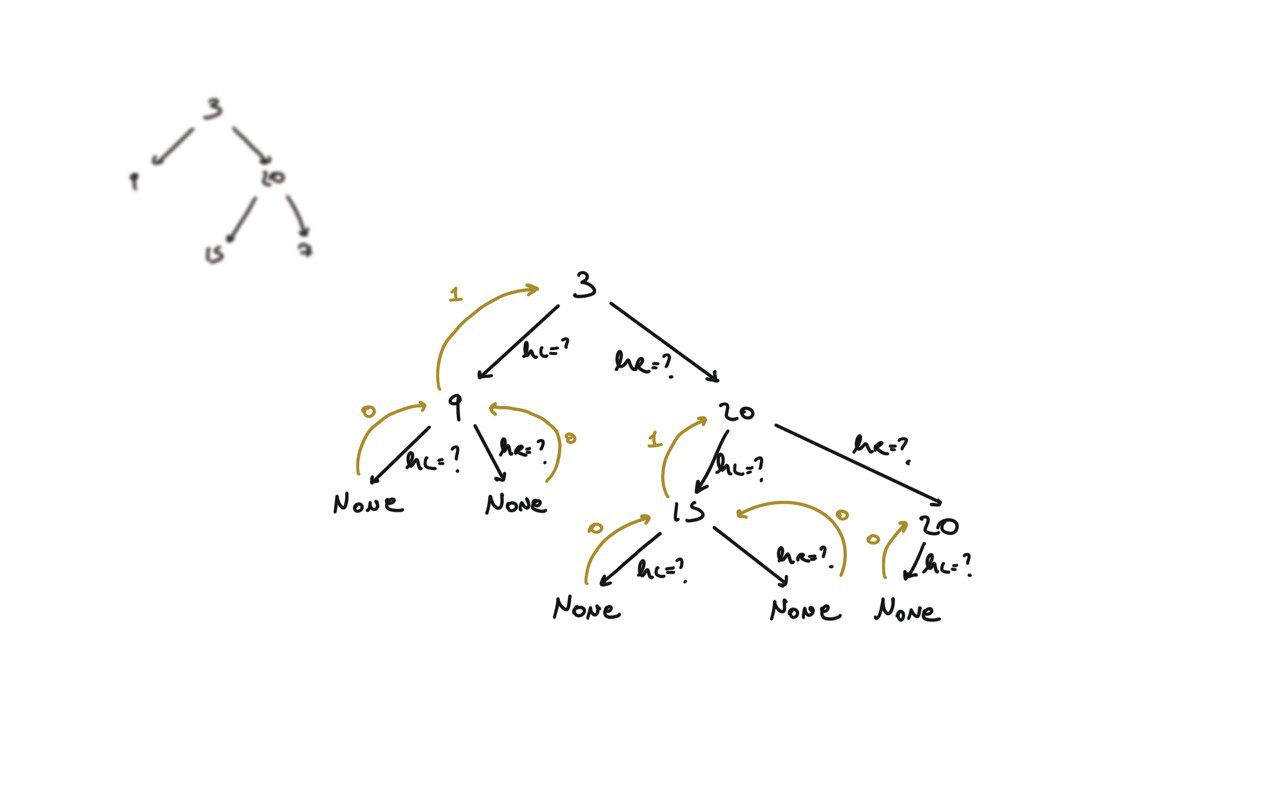
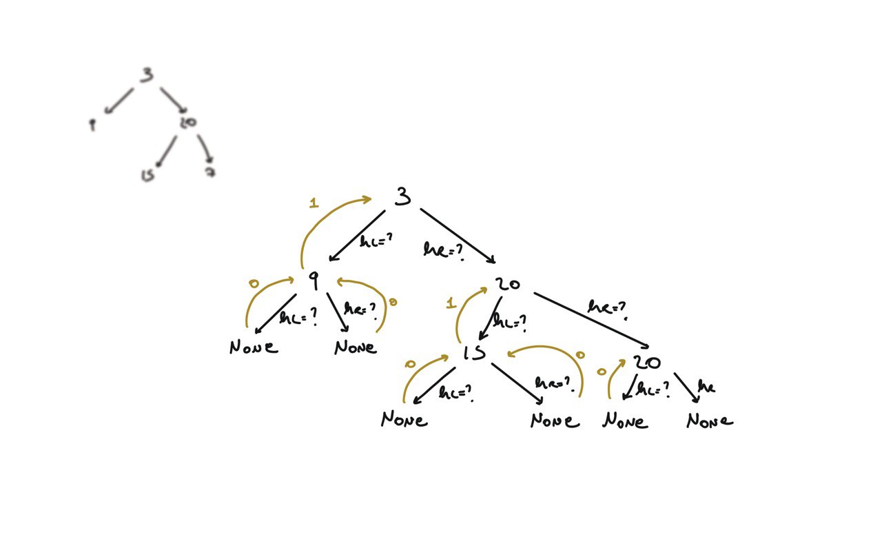
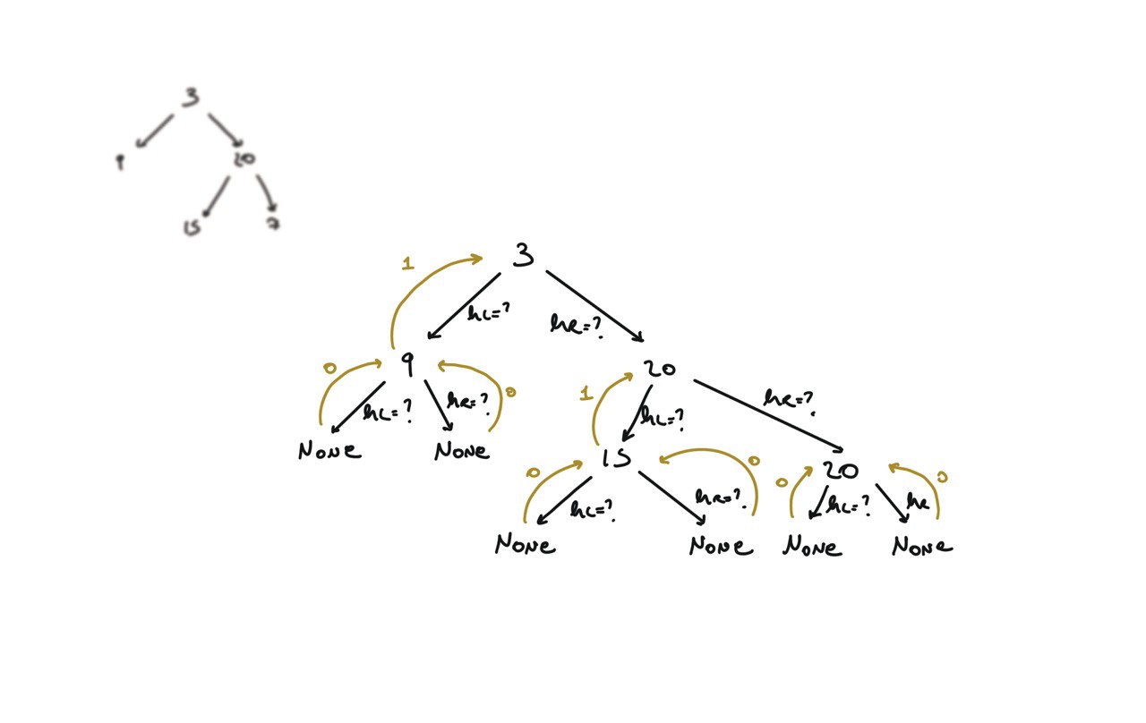
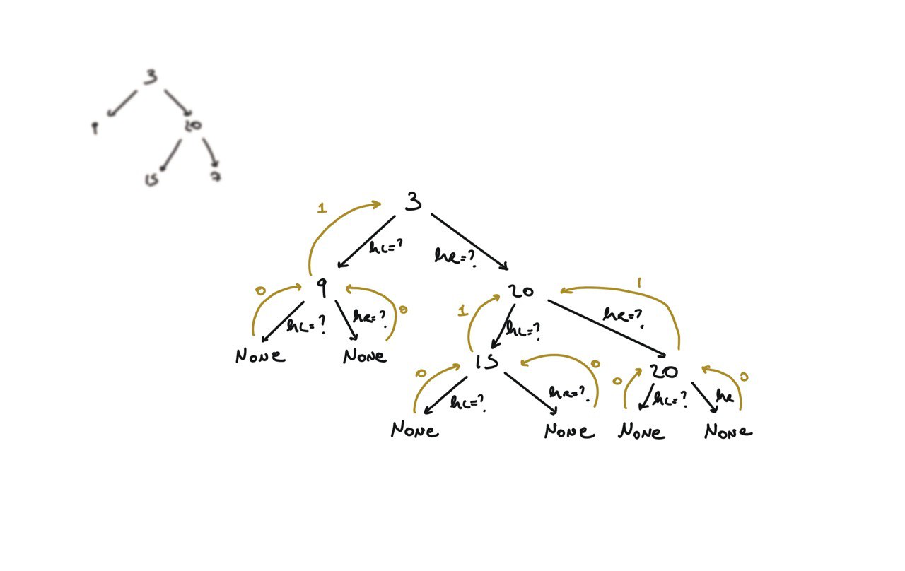
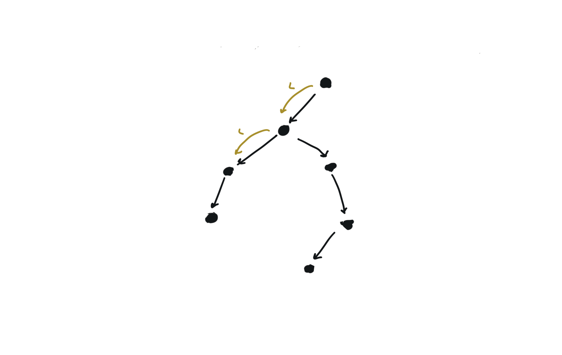
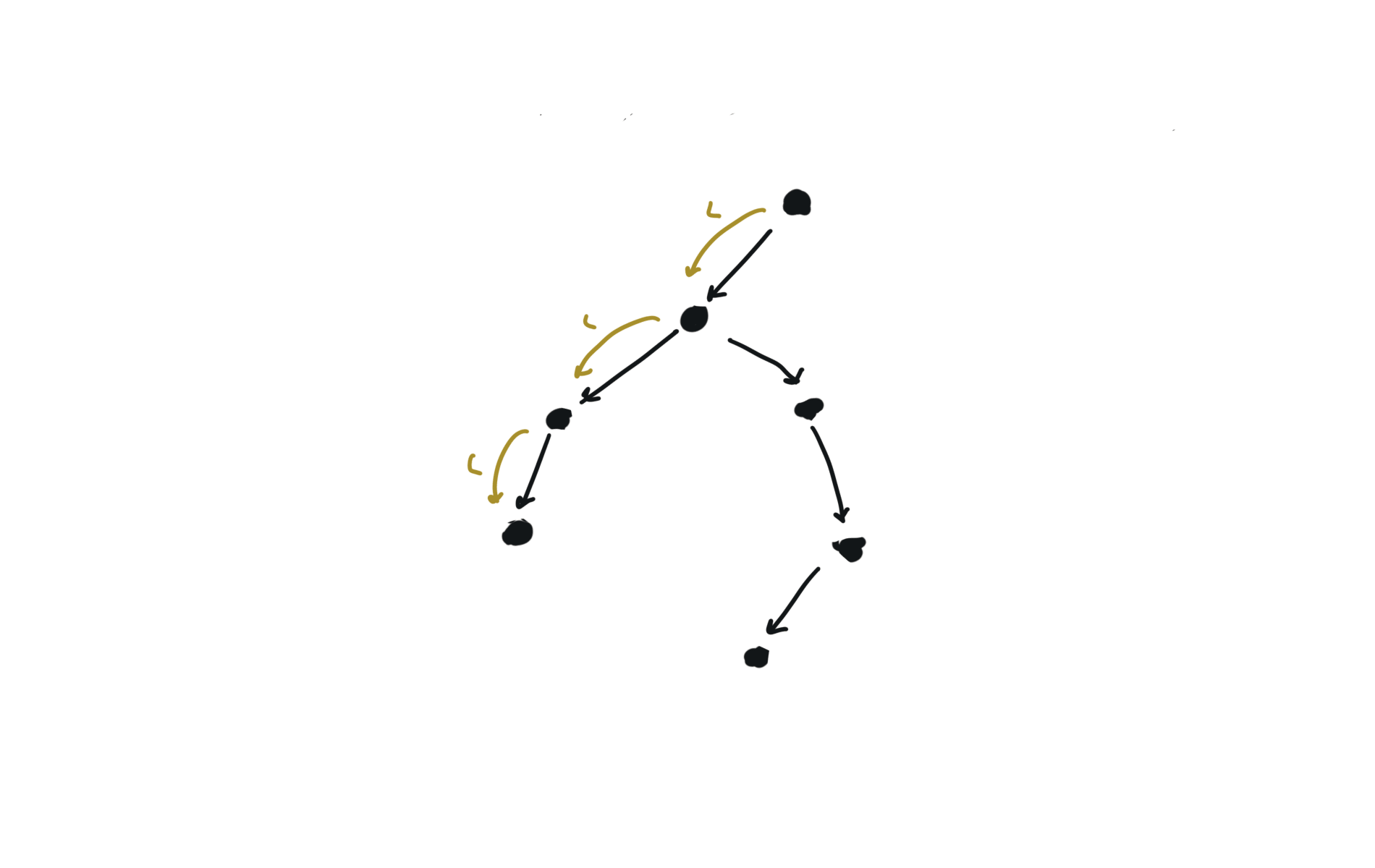
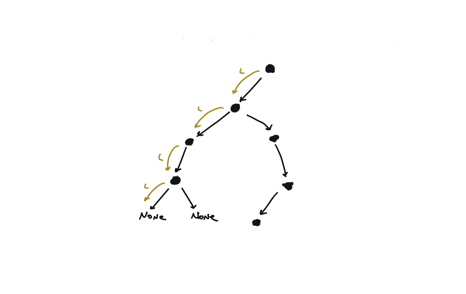
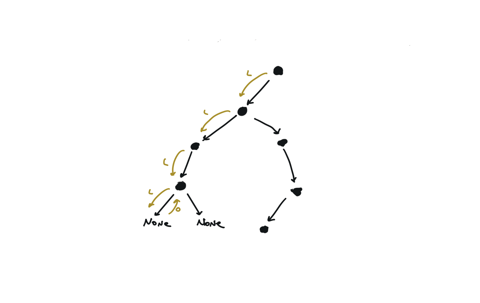
DFS
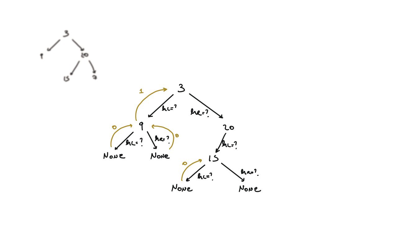
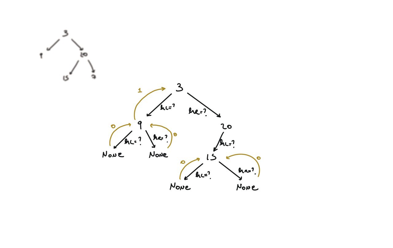
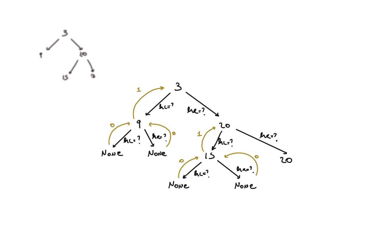
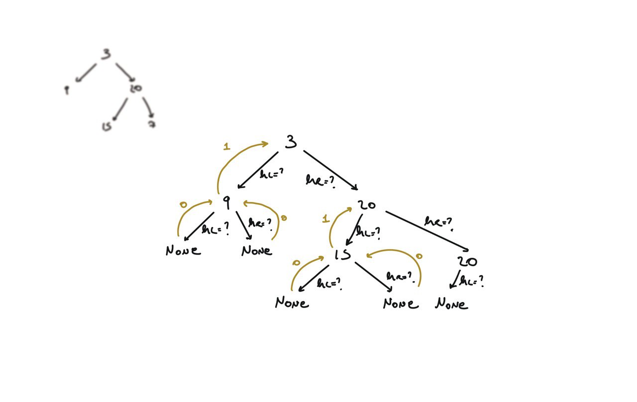
def dfs(root):
	if not root:
		return
	hl = dfs(root.left)
	hr = dfs(root.right)
	return
visualization
BFS
q = deque([root])
while q:
	v = q.popleft()
	if v.left:
		q.append(v.left)
	if v.right:
		q.append(v.right)
visualization
DFS iterative
q = []
while q:
	v = q.pop()
	if v.right:
		q.append(v.right)
	if v.left:
		q.append(v.left)
visualization
time and space complexity
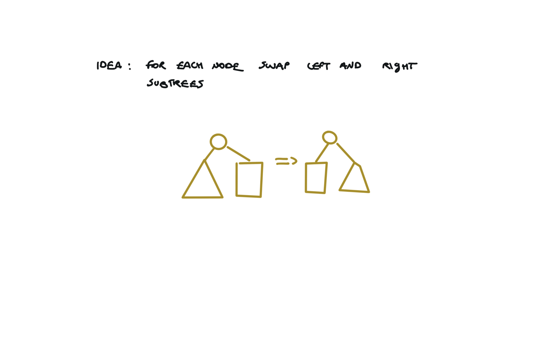
226. Invert Binary Tree
[desc]
(link)
def invertTree(self, root):
    if not root:
        return
    root.left, root.right = root.right,root.left
    self.invertTree(root.left)
    self.invertTree(root.right)
    return root
visualization
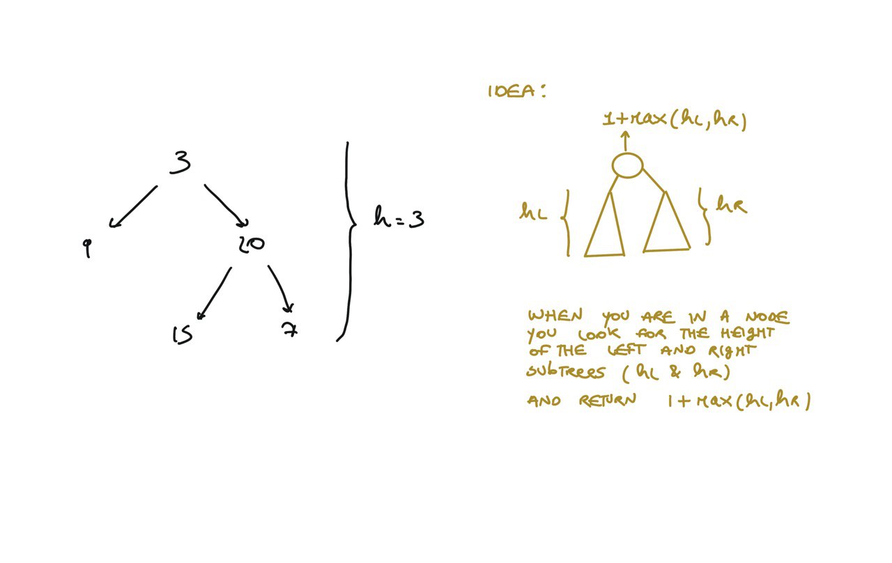
104. Maximum Depth of Binary Tree
[desc]
(link)
def dfs(root):
	if not root:
		return 0
	hl = dfs(root.left)
	hr = dfs(root.right)
	return 1 + max(hl, hr)
return dfs(root)
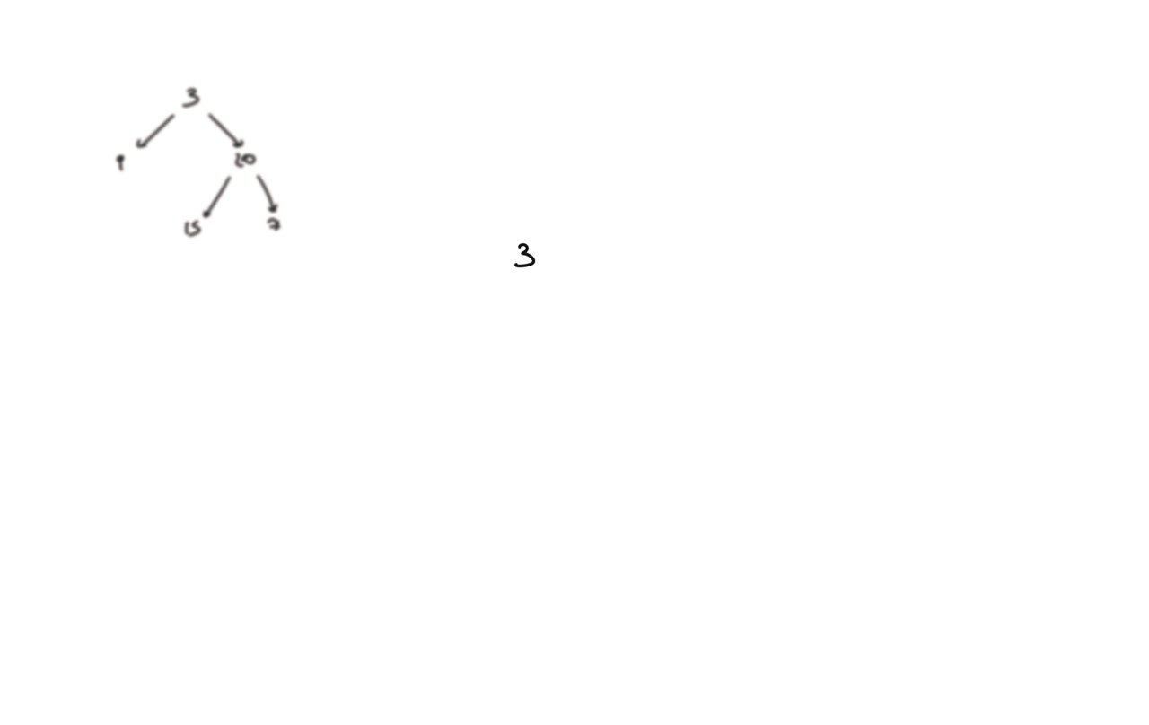
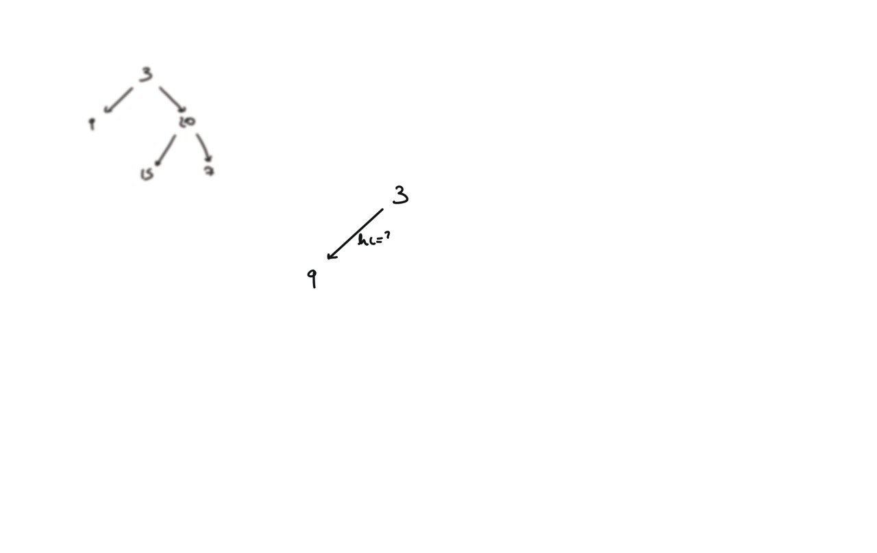
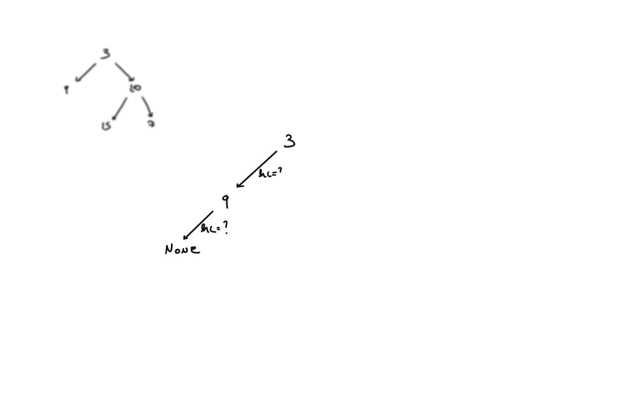
visualization
BFS solution
q = deque([root])
level = 0
while q:
	for i in range(len(q)):
		v = q.popleft()
		if v.left:
			q.append(v.left)
		if v.right:
			q.append(v.right)
	level += 1
return level
110. Balanced Binary Tree
[desc]
(link)
def dfs(root):
    if not root:
        return (True,0)
    b1,h1 = dfs(root.left)
    b2,h2 = dfs(root.right)
    if b1 and b2 and abs(h1-h2)<=1:
        return (True,max(h1,h2)+1)
    else:
        return (False,max(h1,h2)+1)
return dfs(root)[0]
100. Same Tree
[desc]
(link)
def dfs(root1,root2):
    if not root1 and not root2:
        return True
    if not root1 and root2:
        return False
    if root1 and not root2:
        return False
    a = dfs(root1.left,root2.left)
    b = dfs(root1.right,root2.right)
	return root1.val == root2.val and a and b
return dfs(p,q)
if not root1 and not root2:
    return True
if not root1 and root2:
    return False
if root1 and not root2:
    return False
root1
root2
output i want
T
T
nothing
T
F
F
F
T
F
F
F
T
if not root1 or not root2:
	return root1 == root2
Another way to do it
def dfs(root1,root2):
    if not root1 and not root2:
        return True
    if not root1 and root2:
        return False
    if root1 and not root2:
        return False
    if root1.val != root2.val:
        return False
    a = dfs(root1.left,root2.left)
    b = dfs(root1.right,root2.right)
    return  a and b
return dfs(p,q)
572. Subtree of Another Tree
[desc]
(link)
def sameTree(root1,root2):
    if not root1 and not root2:
        return True
    if not root1 and root2:
        return False
    if not root2 and root1:
        return False
    l = sameTree(root1.left, root2.left)
    r = sameTree(root1.right, root2.right)
    return l and r and root1.val == root2.val

def dfs(root,subRoot)->bool:
    if not root:
        return False
    if sameTree(root, subRoot):
        return True
    l = dfs(root.left, subRoot)
    r = dfs(root.right, subRoot)
    return l or r
return dfs(root,subRoot)
102. Binary Tree Level Order Traversal
[desc]
(link)
if not root:
    return []
q = deque([root])
out = []
while q:
    elem = []
    for i in range(len(q)):
        e = q.popleft()
        if e.left:
            q.append(e.left)
        if e.right:
            q.append(e.right)
        elem.append(e.val)
    out.append(elem)
return out
199. Binary Tree Right Side View
[desc]
(link)
if not root:
    return
d = deque([root])
out = []
while d:
    l = []
    for i in range(len(d)):
        n = d.popleft()
        if n.left:
            d.append(n.left)
        if n.right:
            d.append(n.right)
        l.append(n.val)
    out.append(l[-1])
return out
543. Diameter of Binary Tree
[desc]
(link)
diameter = [0]
def dfs(root):
    if not root:
        return 0
    l = dfs(root.left)
    r = dfs(root.right)
    diameter[0] = max(diameter[0],l+r)
    return 1+ max(l,r)
dfs(root)
return diameter[0]
visualization
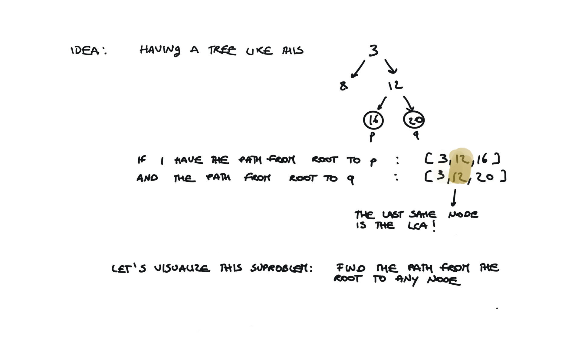
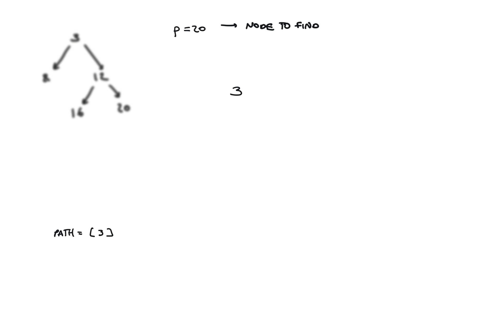
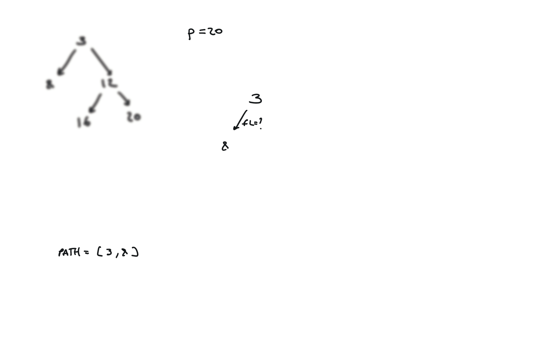
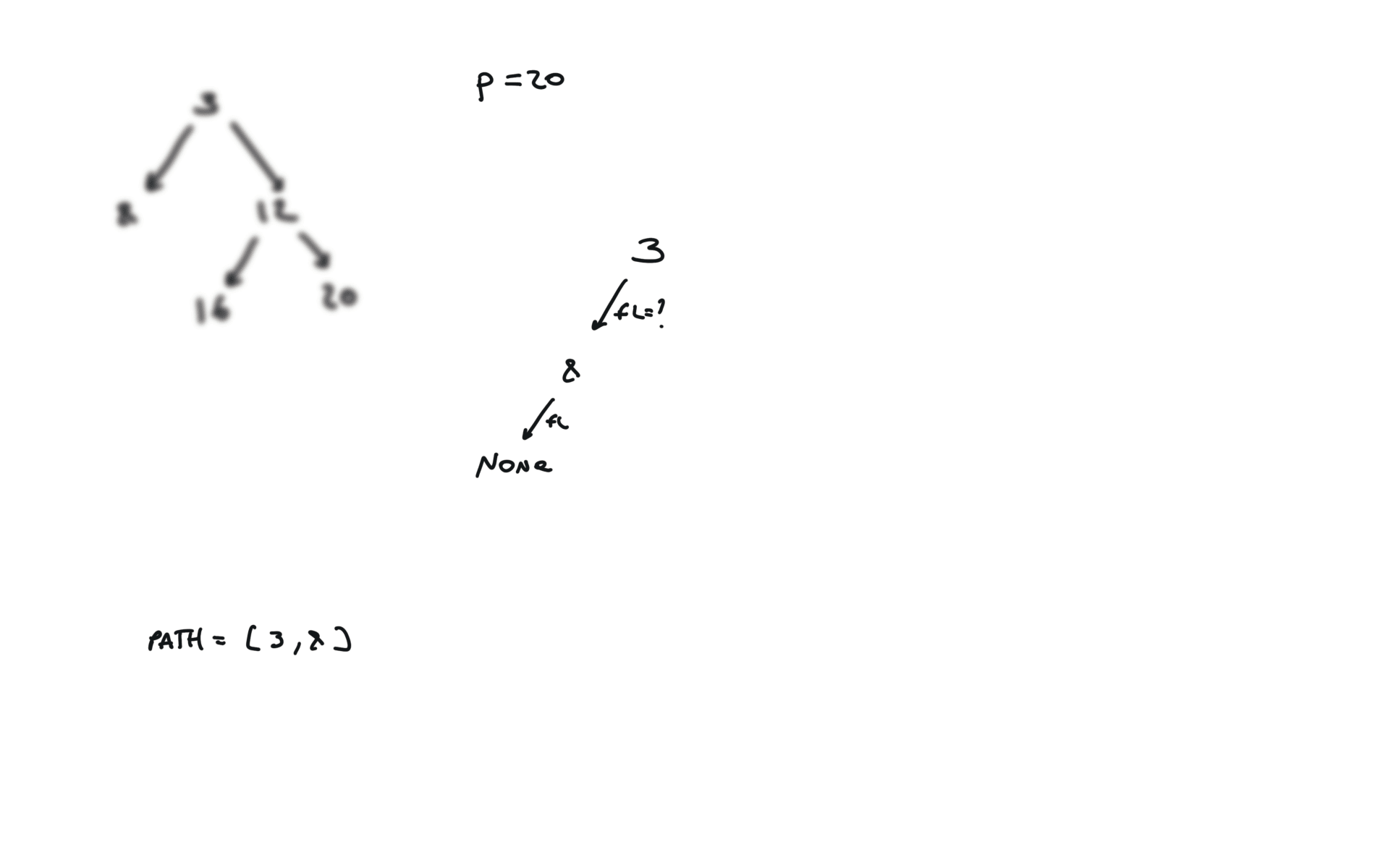
236. lowest-common-ancestor-of-a-binary-tree
[desc]
(link)
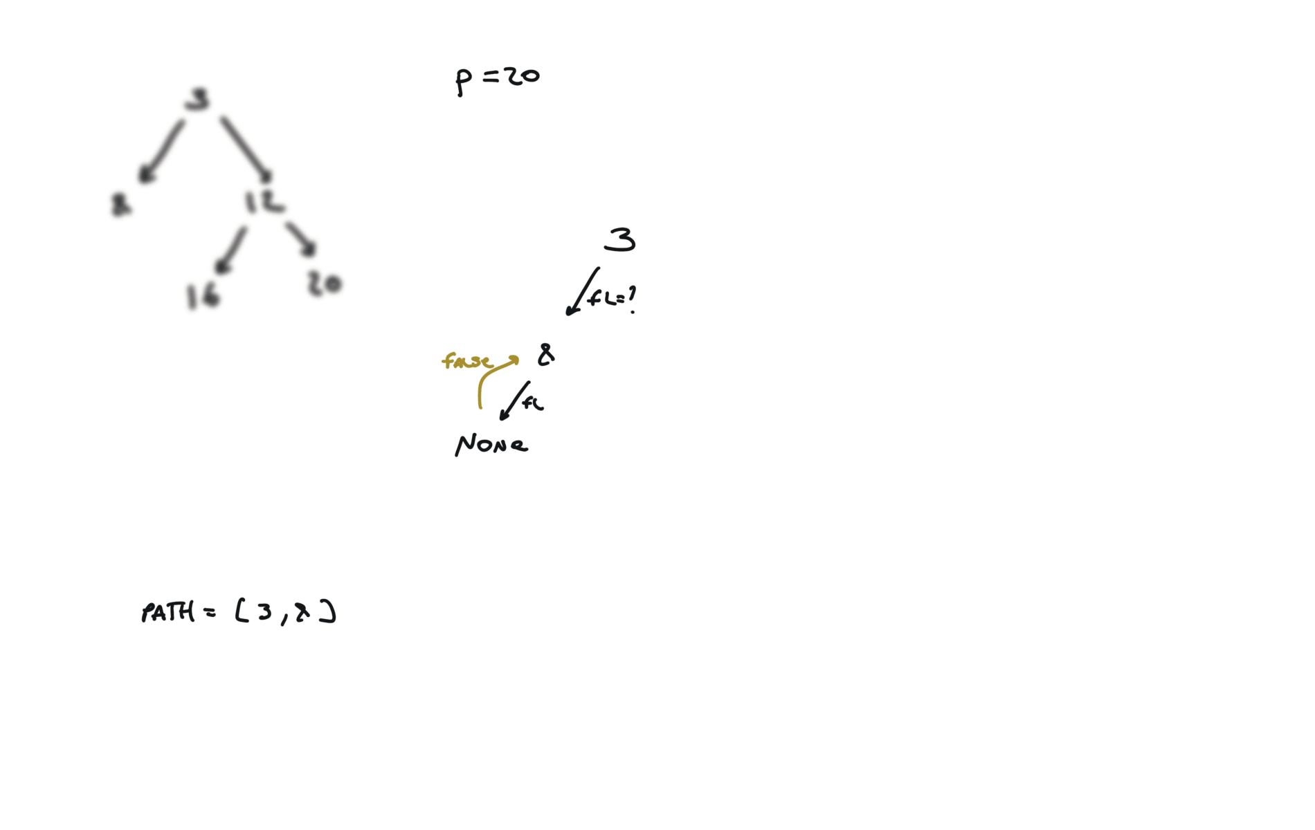
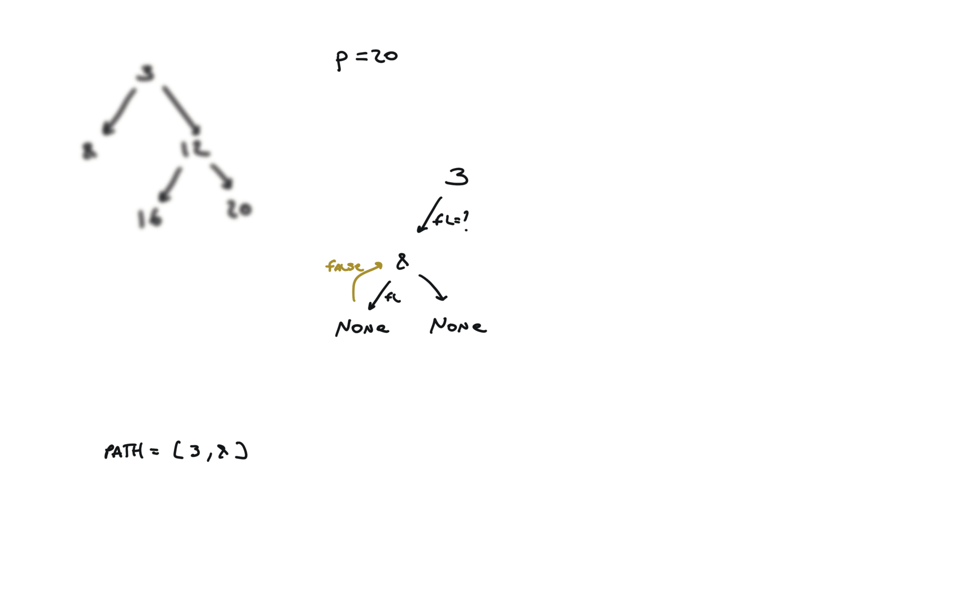
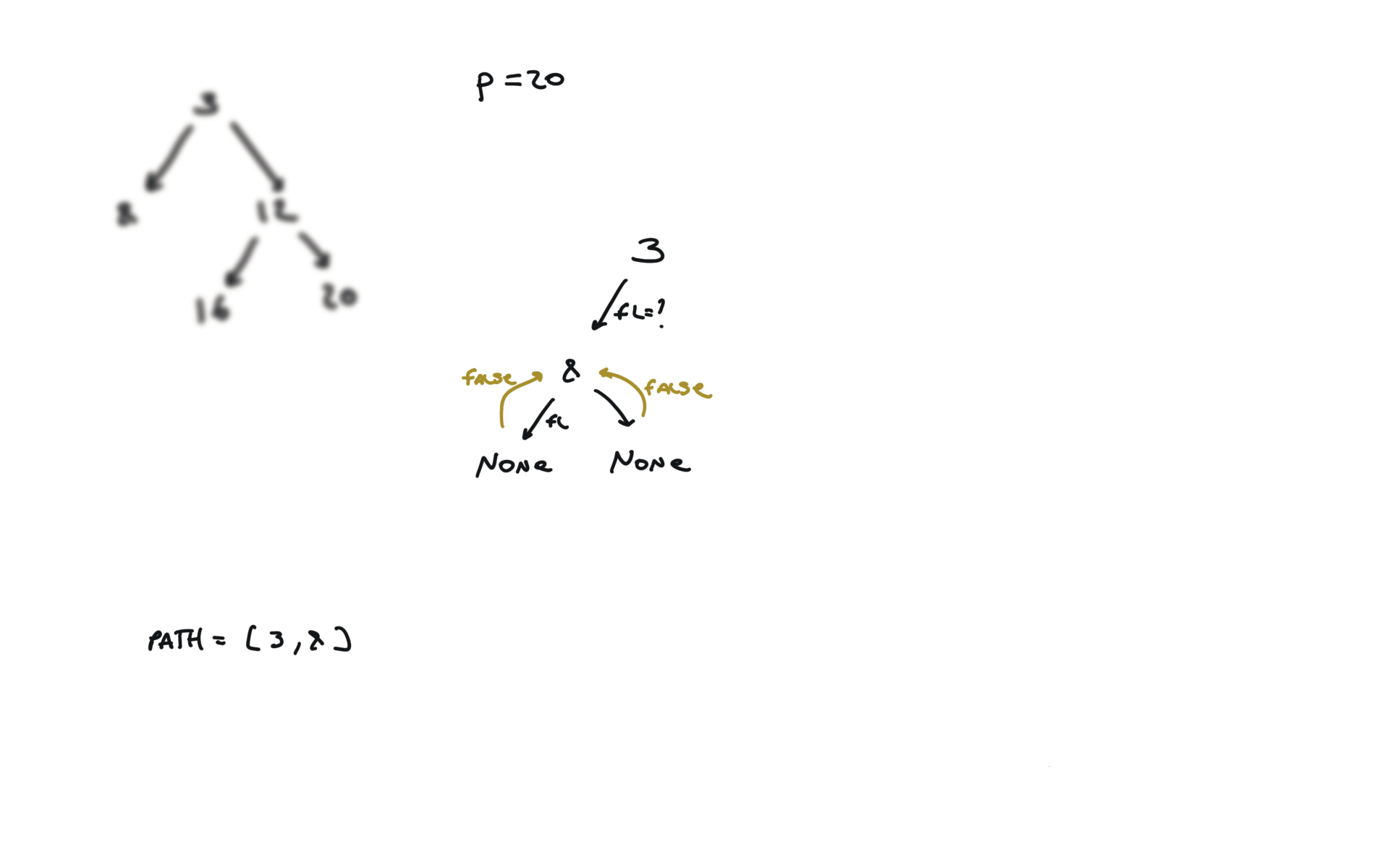
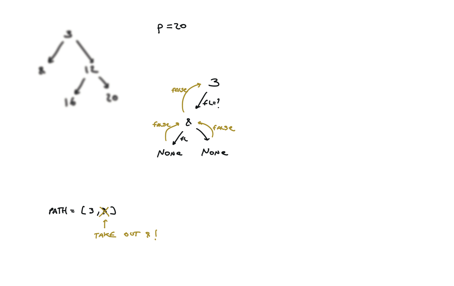
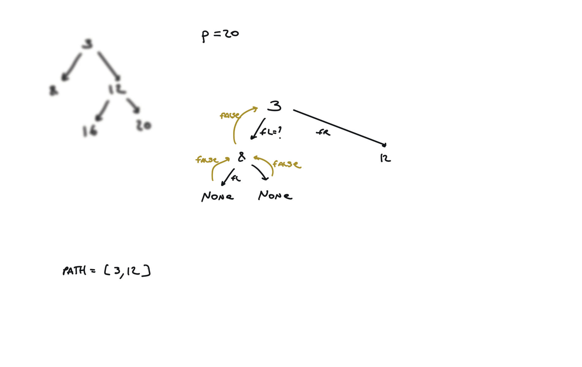
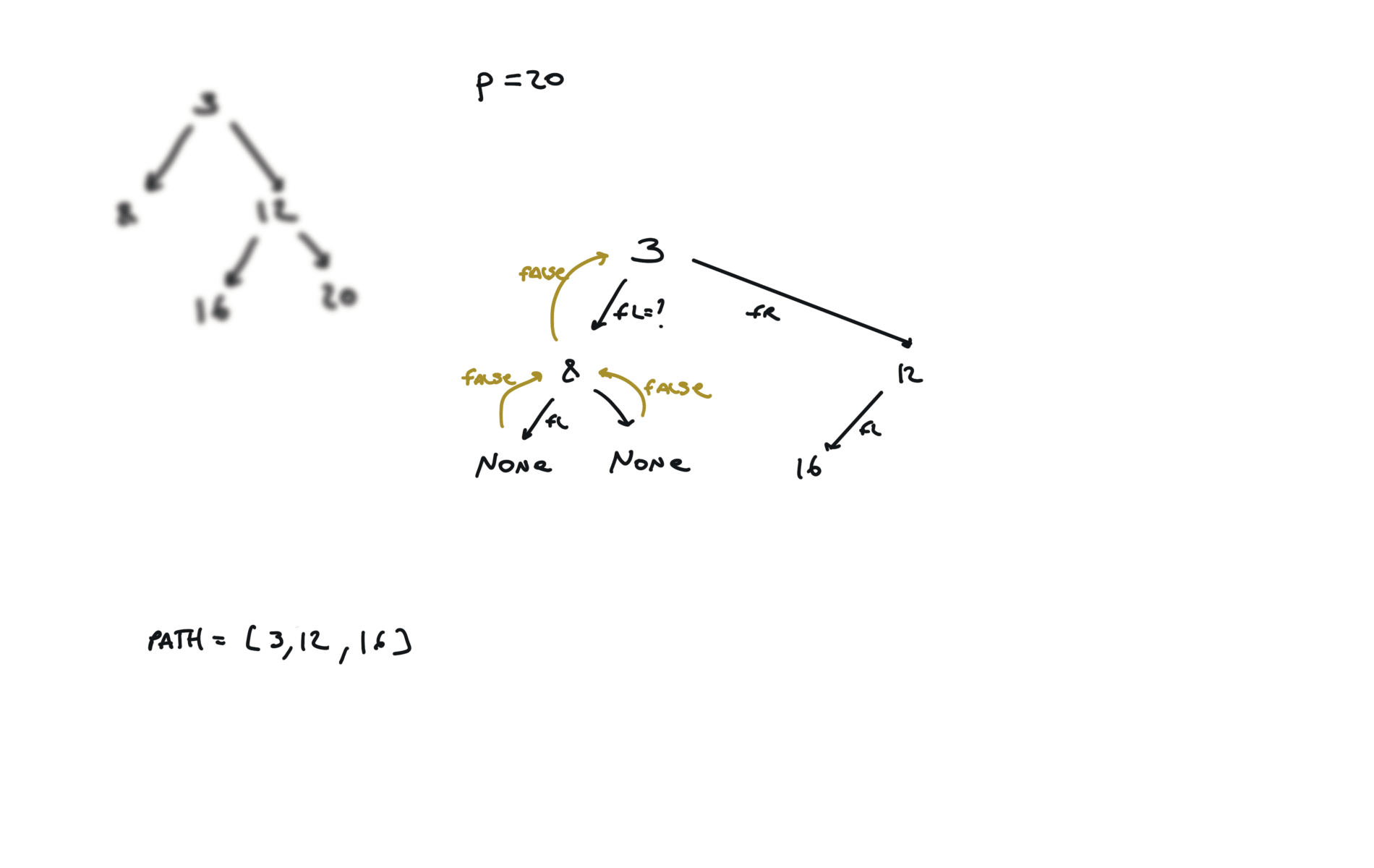
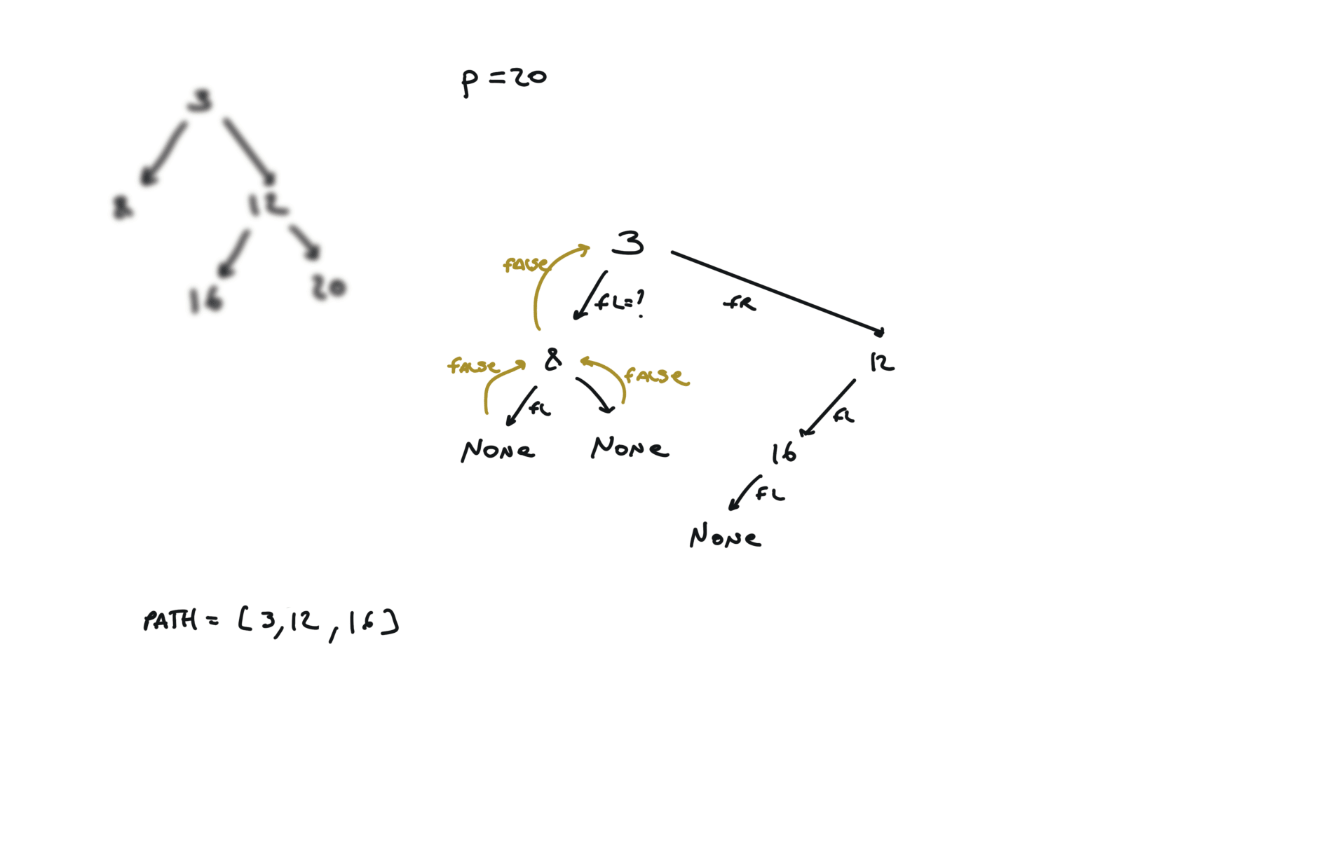
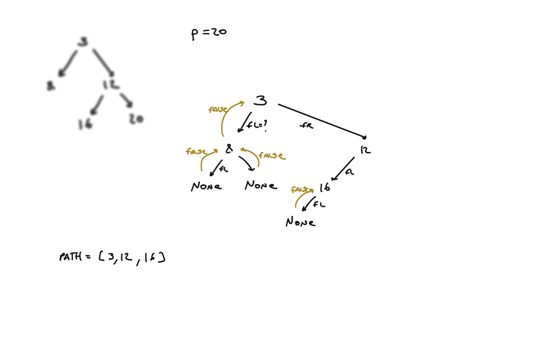
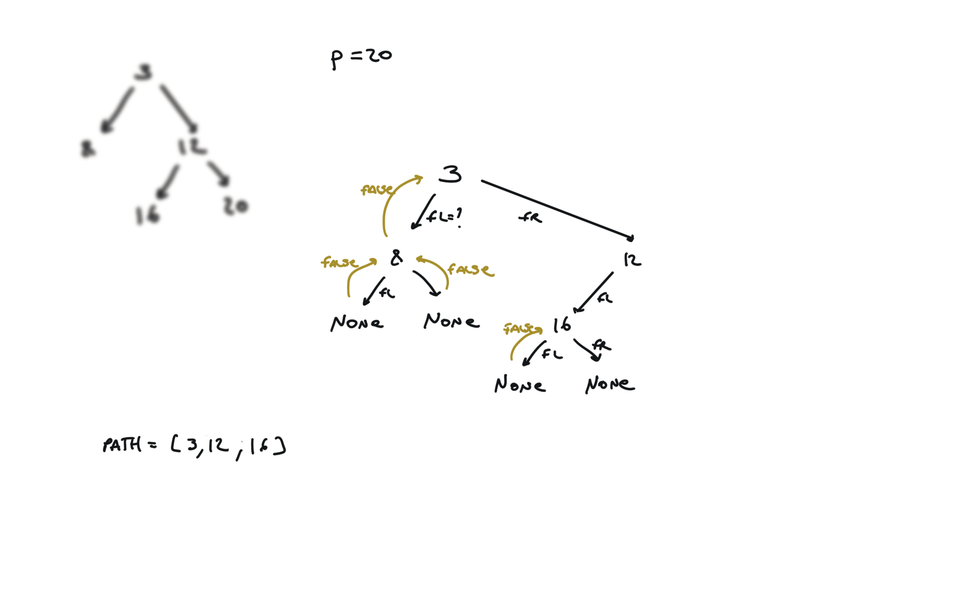
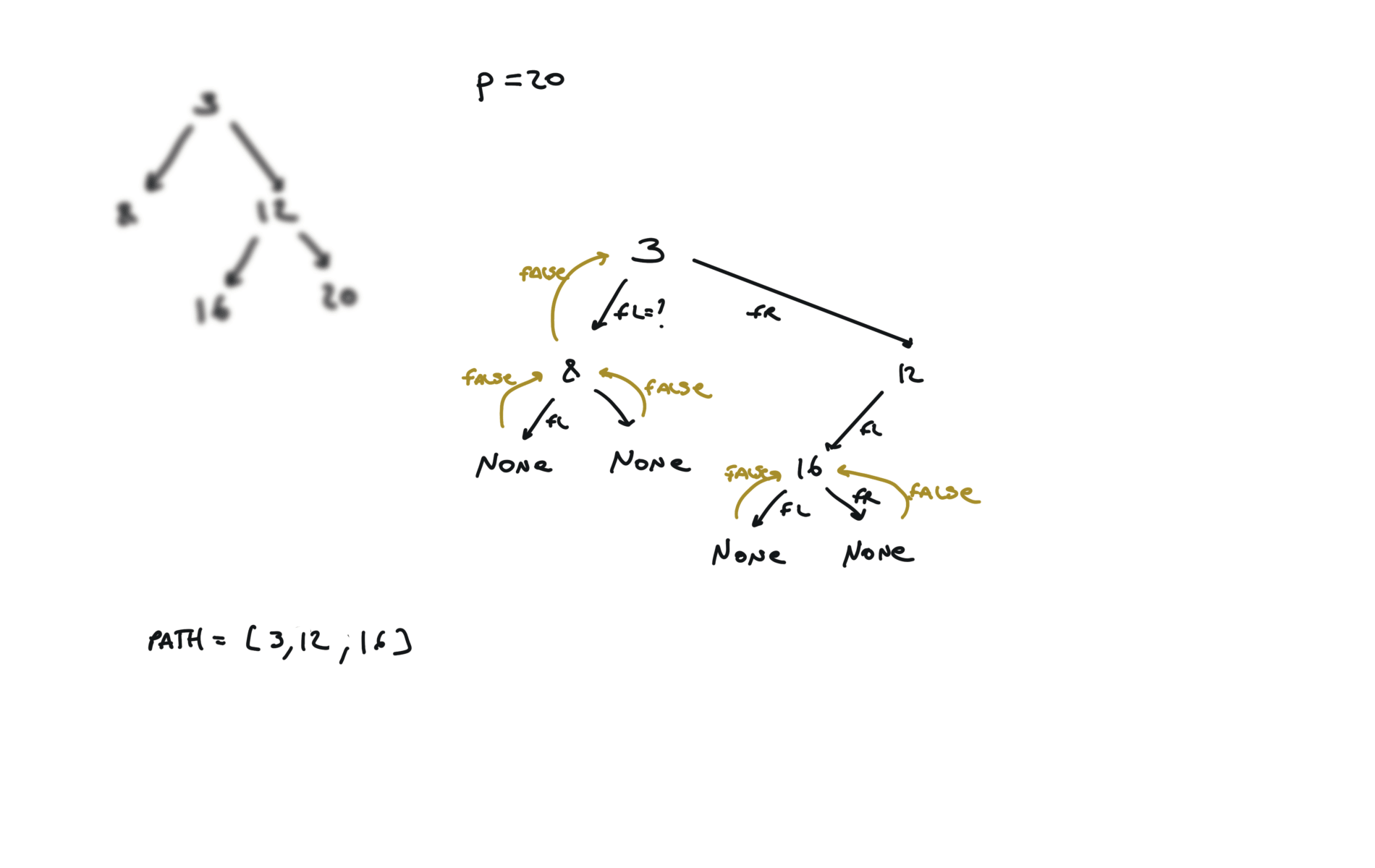
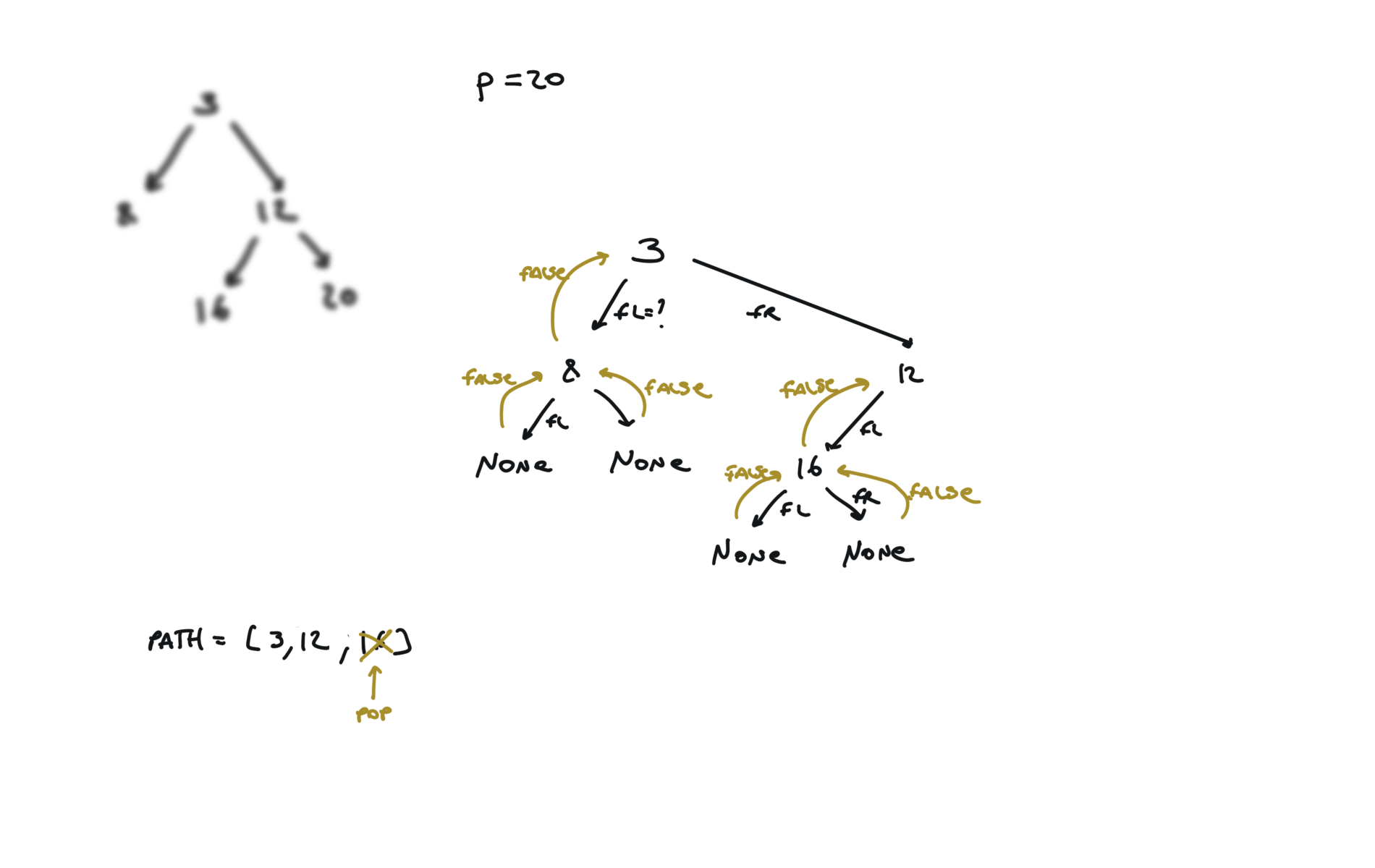
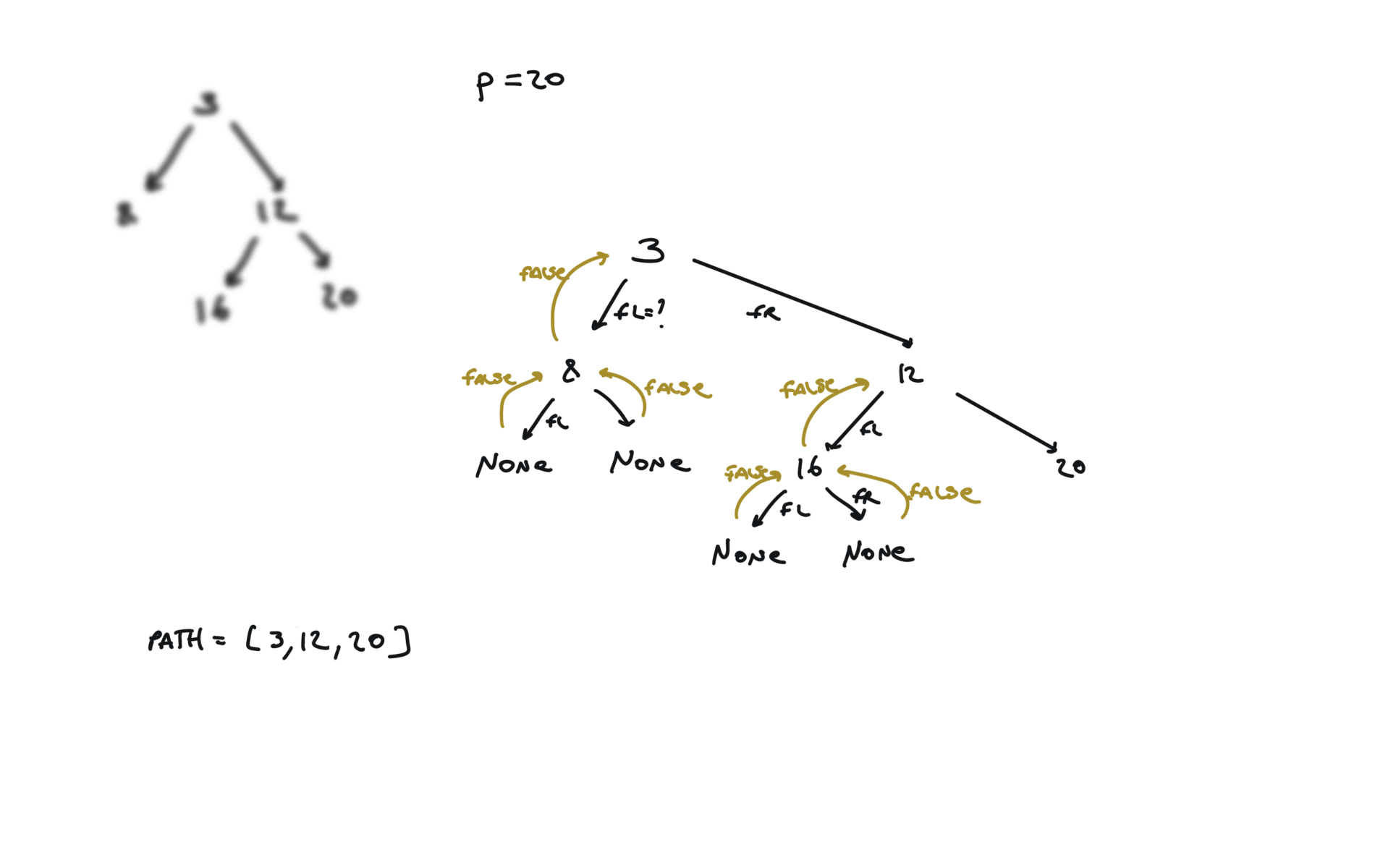
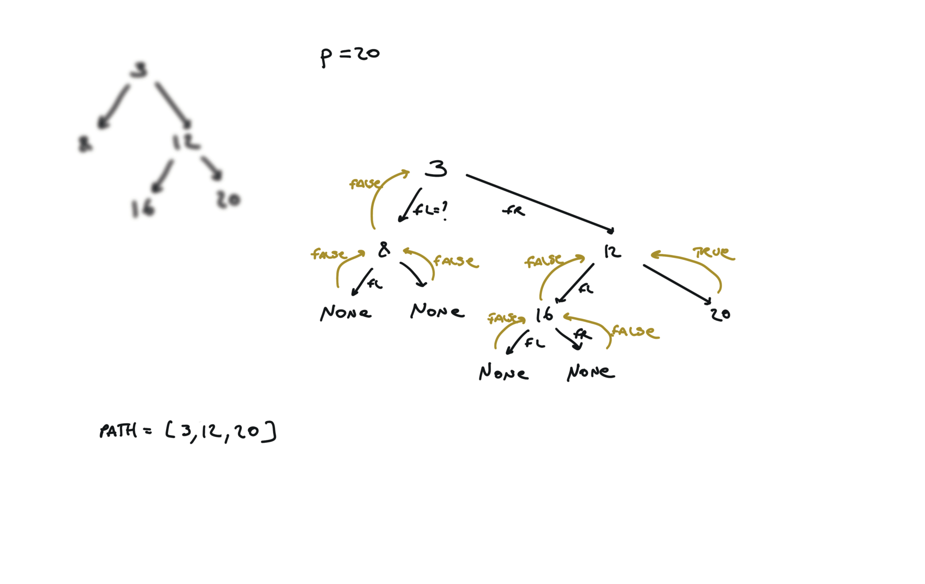
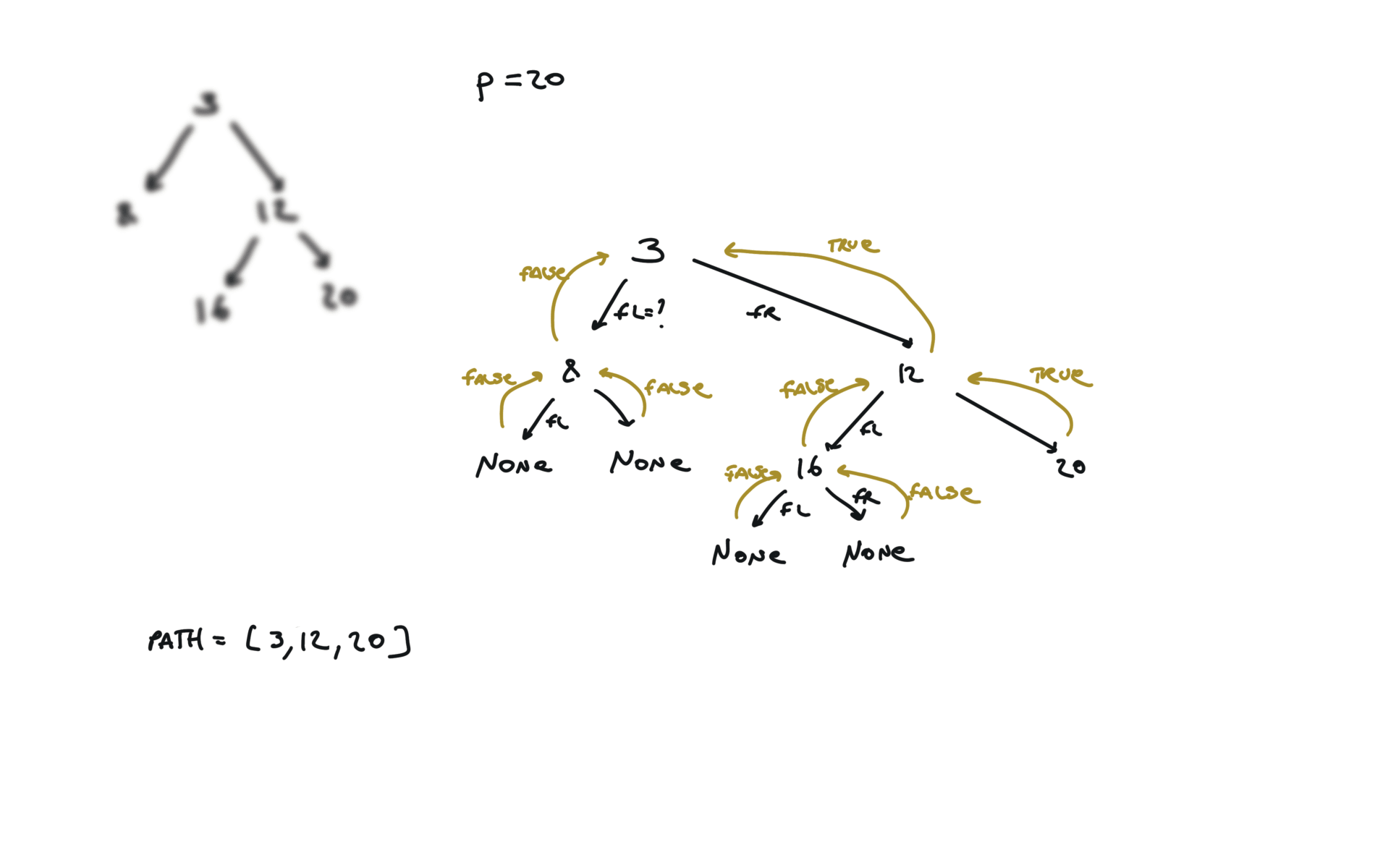
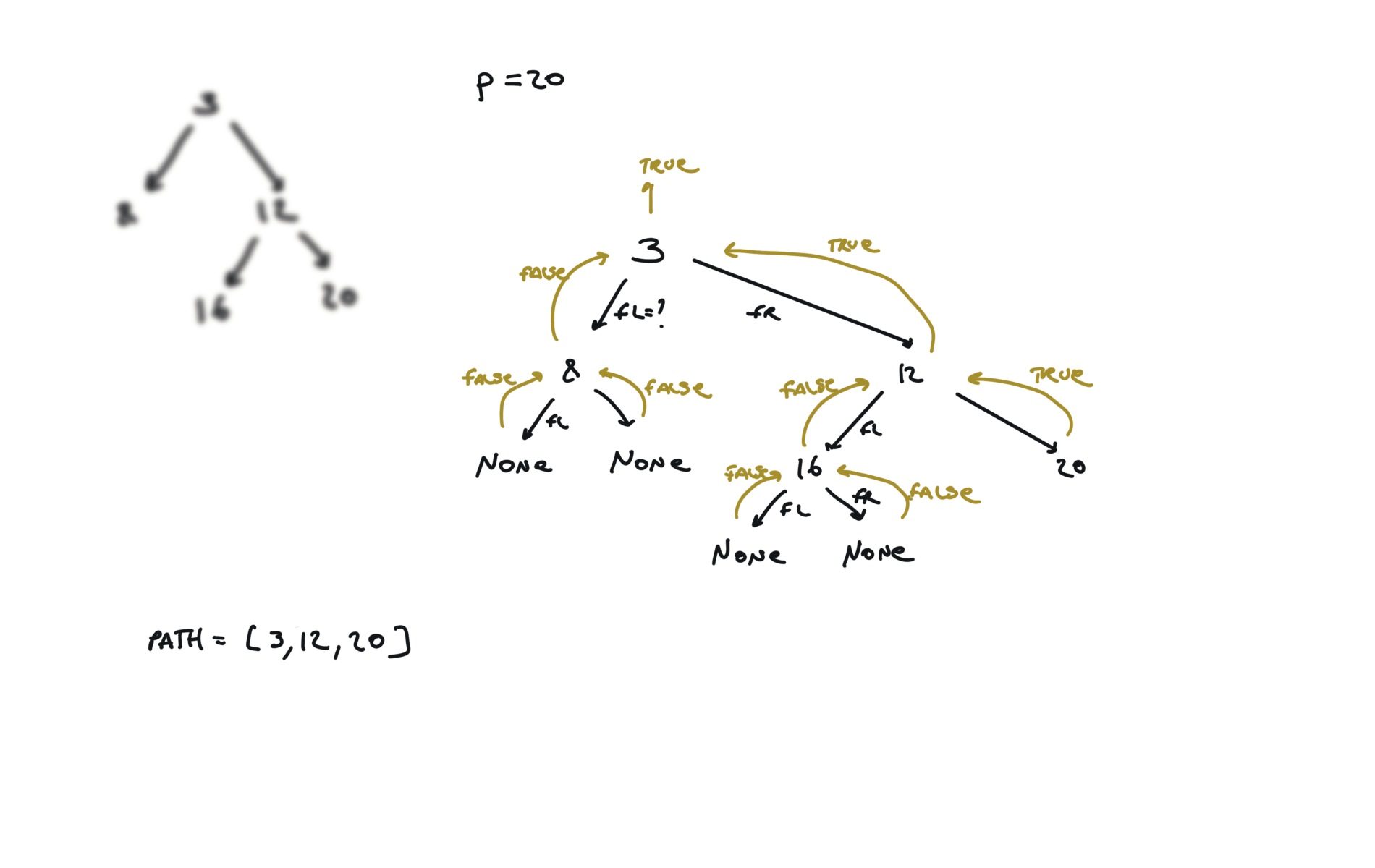
def dfs(root, v, path):
	if not root:
        return False
    path.append(root.val)
    if root.val == v:
        return True
    fl = dfs(root.left, v, path)
    if fl:
        return True
    fr = dfs(root.right, v, path)
    if fr:
        return True
    path.pop()
    return False

p1, p2 = [], []
dfs(root,p.val,p1)
dfs(root,q.val,p2)
i = 0
ret = None
while i < len(p1) and i < len(p2):
    if p1[i] != p2[i]:
        break
    ret = p1[i]
    i+=1
return TreeNode(ret)
visualization
617. Merge Two Binary Trees
[desc]
(link)
def dfs(root1, root2):
    if not root1:
        return root2
    if not root2:
        return root1
    tree = TreeNode(root1.val + root2.val)
    tree.left = dfs(root1.left, root2.left)
    tree.right = dfs(root1.right, root2.right)
    return tree
return dfs(root1, root2)
124. Binary Tree Maximum Path Sum
[desc]
(link)
res = [root.val]
def dfs(root):
    if not root:
        return 0
    leftMax = dfs(root.left)
    rightMax = dfs(root.right)
    leftMax = max(leftMax, 0)
    rightMax = max(rightMax, 0)
    res[0] = max(res[0], root.val + leftMax + rightMax)
    return root.val + max(leftMax, rightMax)
dfs(root)
return res[0]
Backtracking
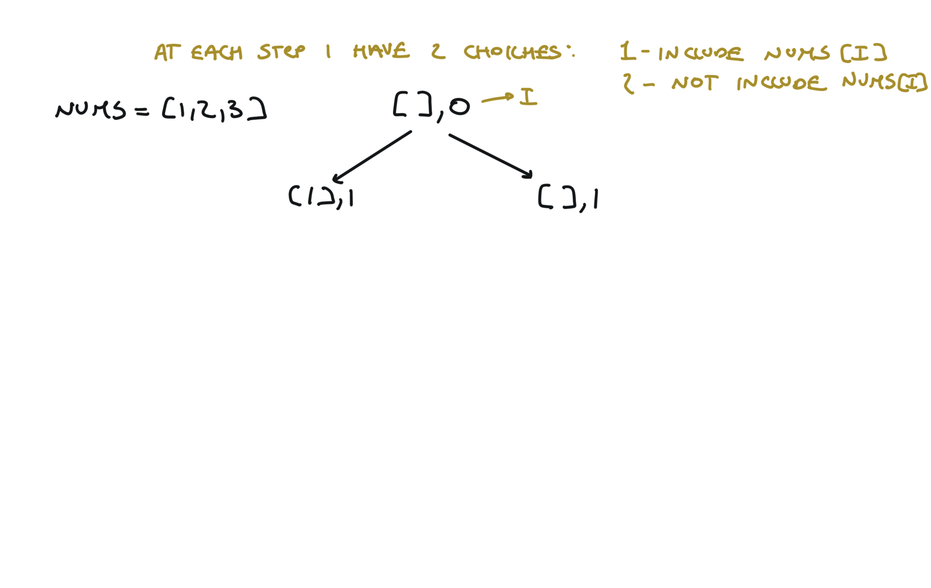
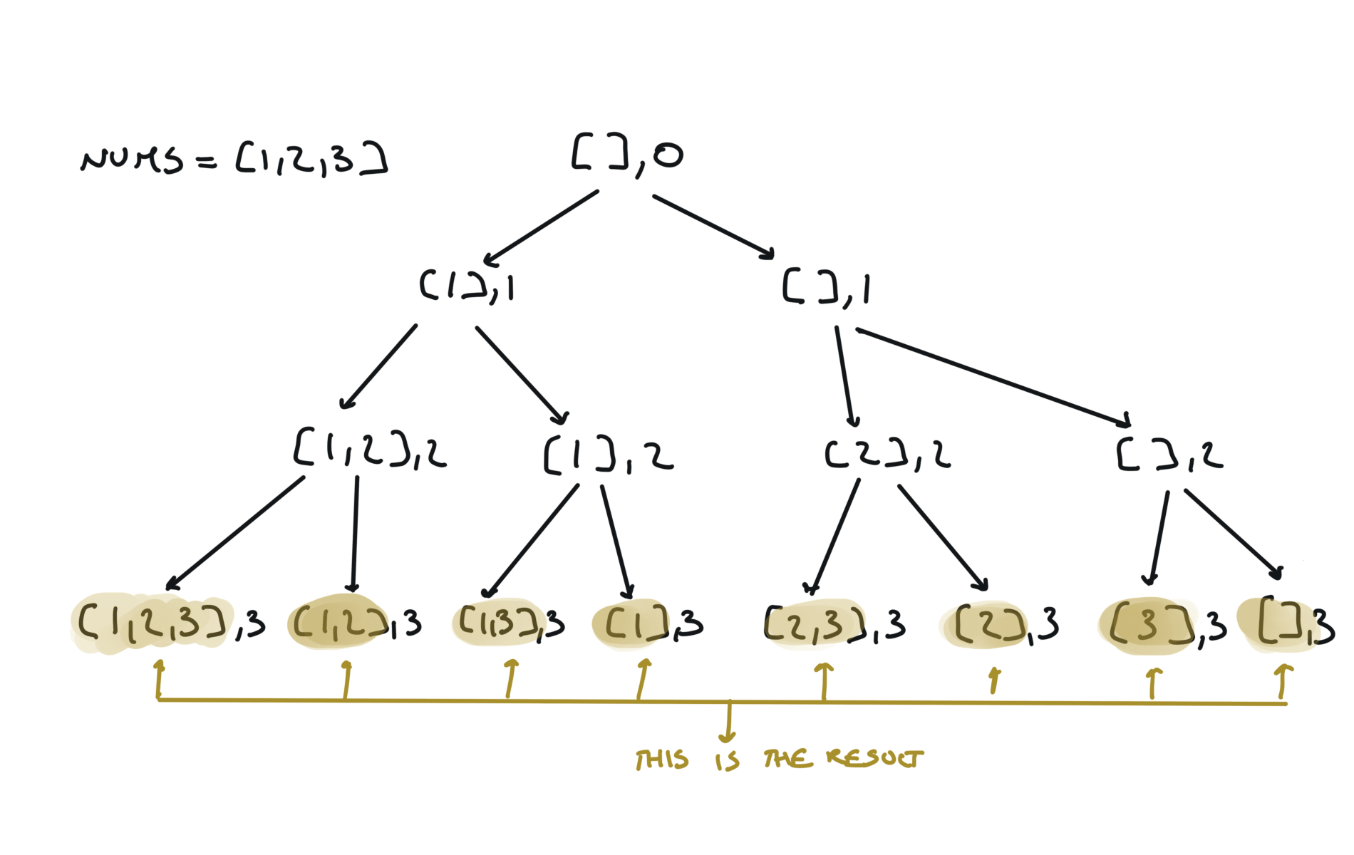
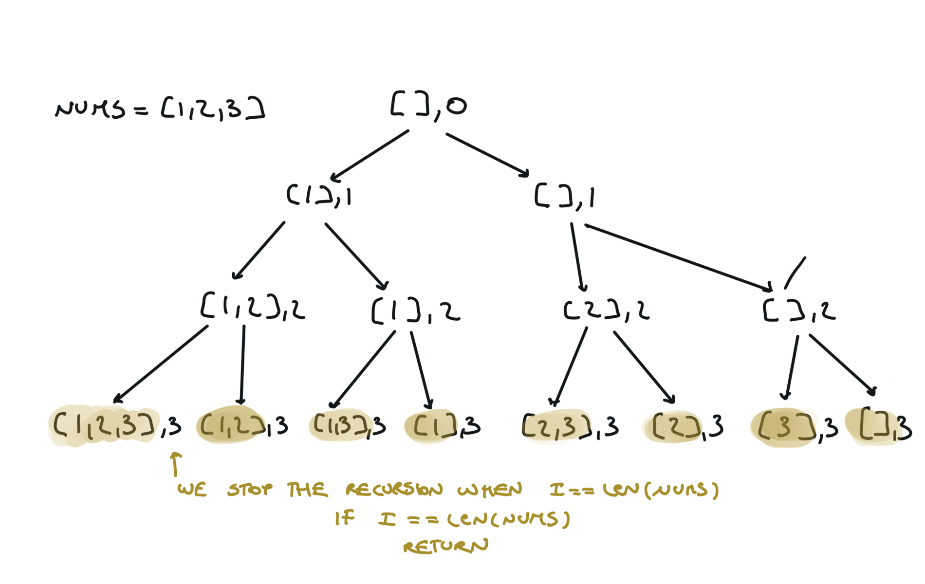
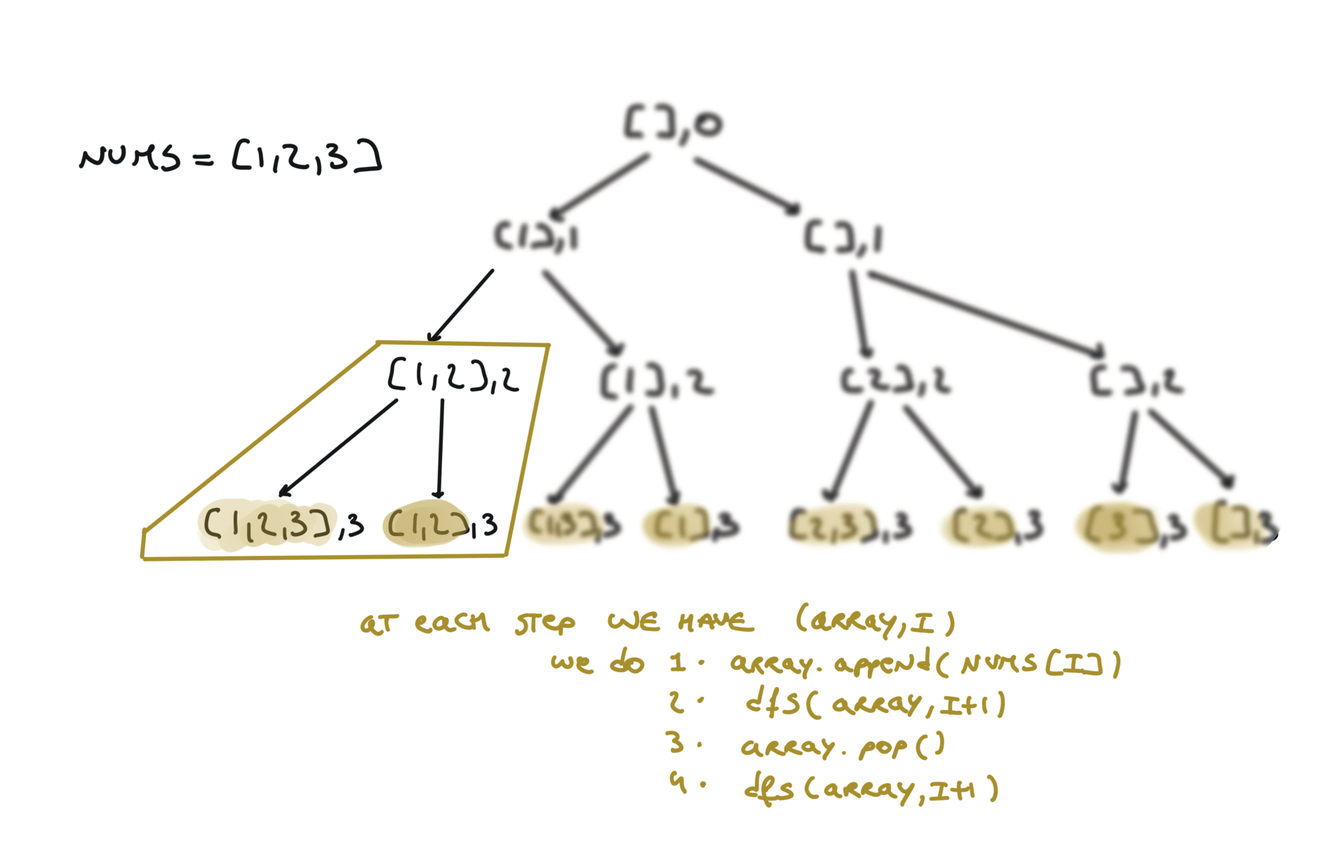
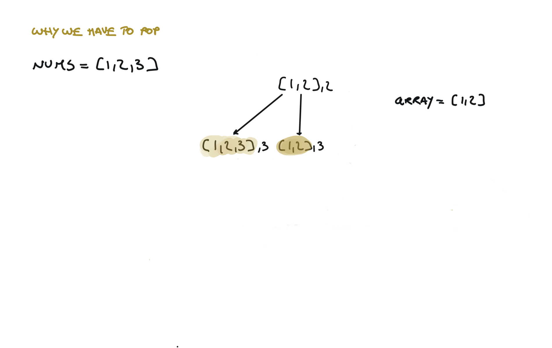
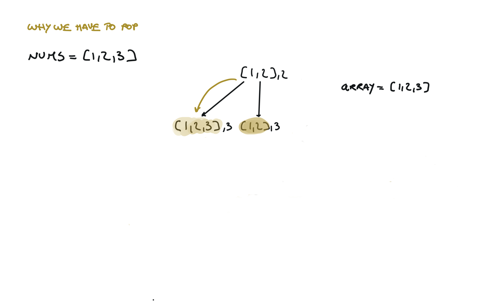
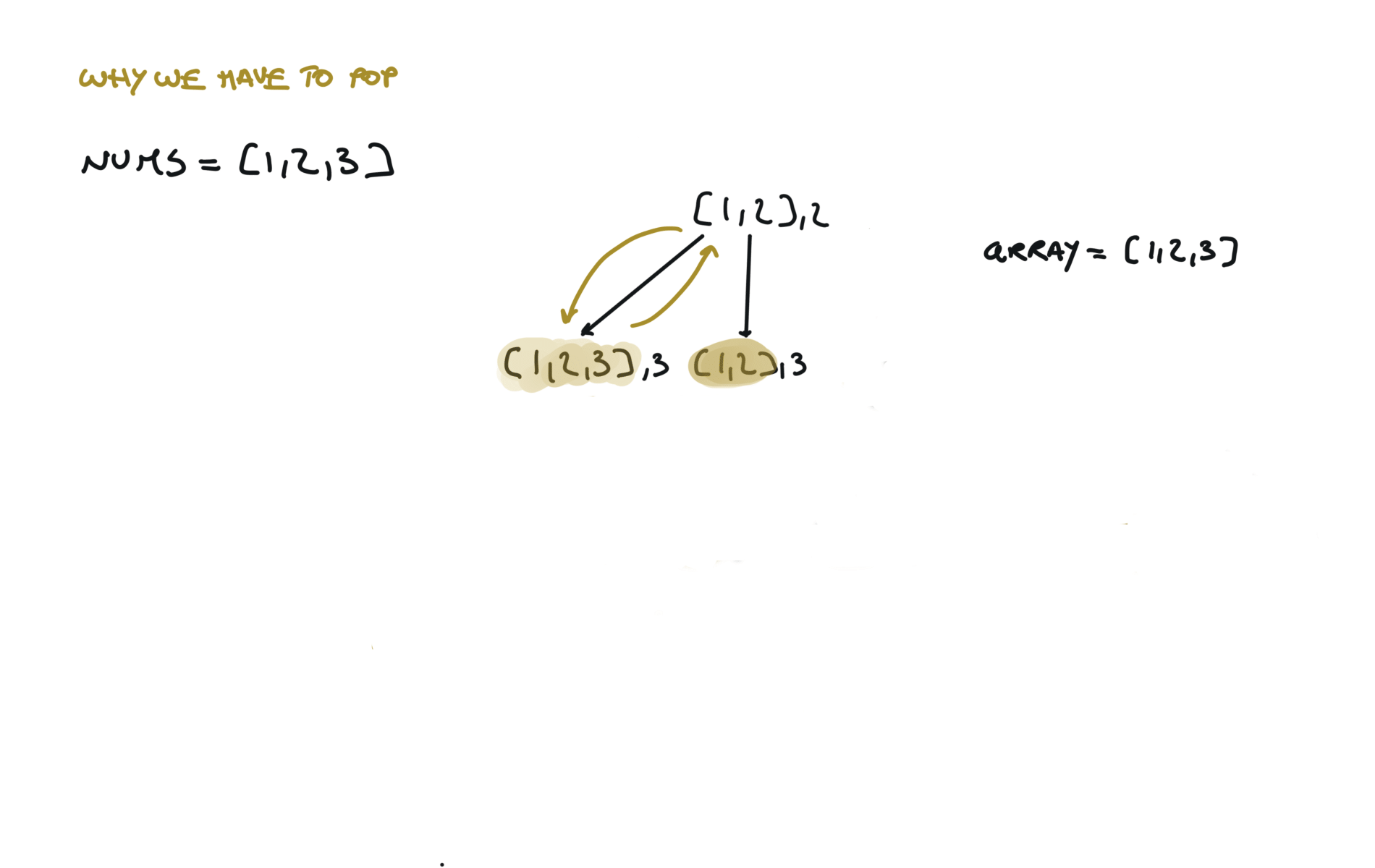
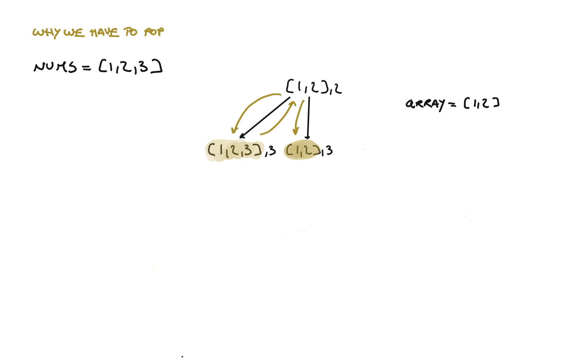
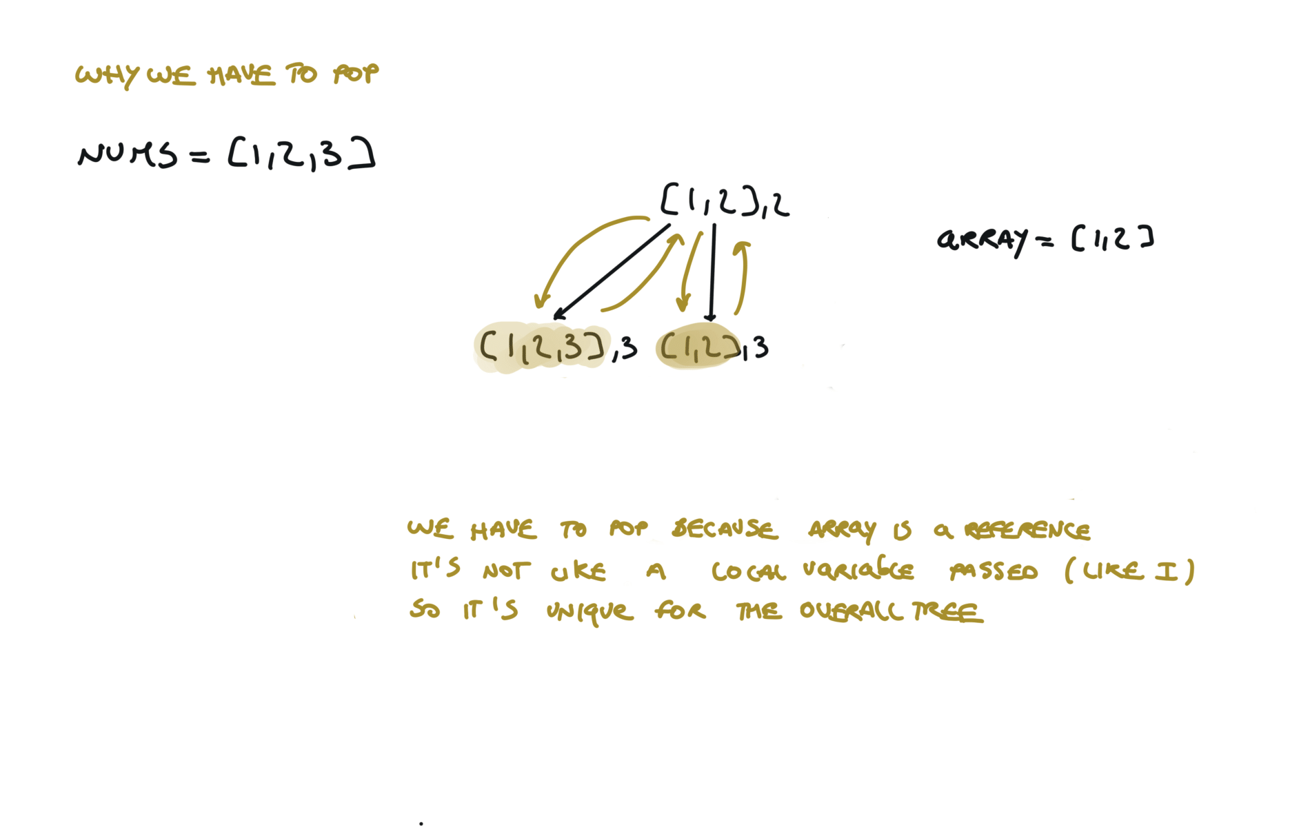
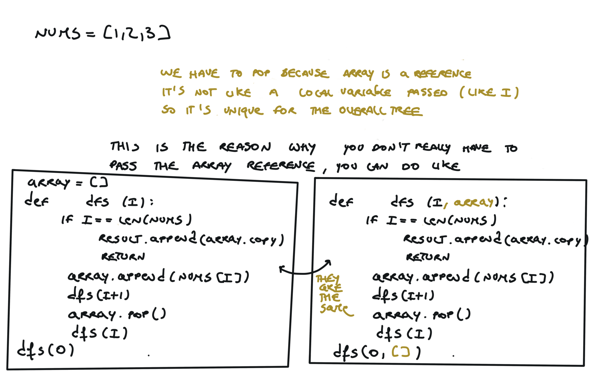
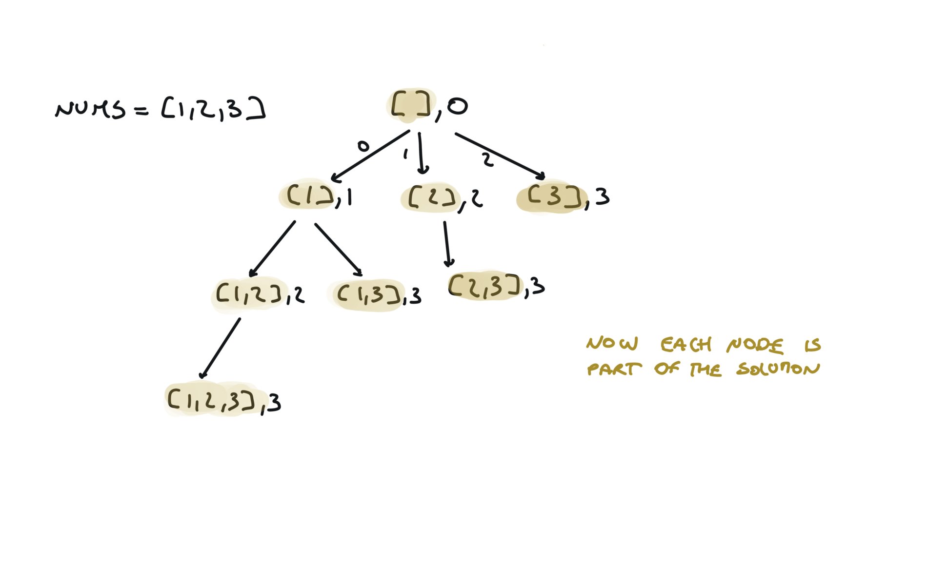
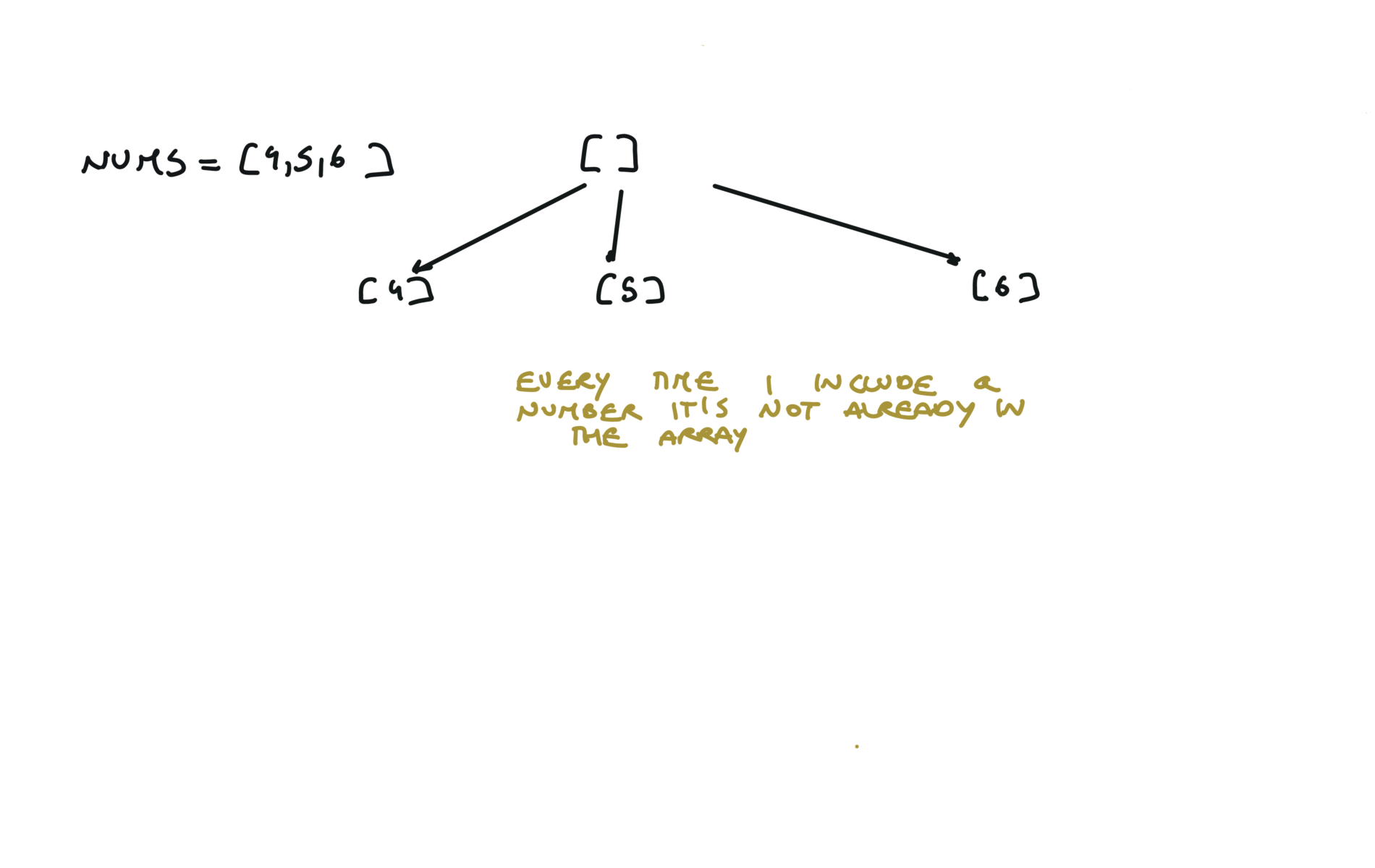
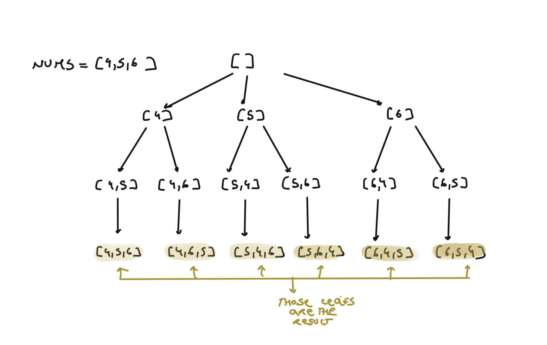
Python is convenient and you can squeeze down the append-recursiveCall-pop to just 1 line, like this: Or view interactive visualization with this link78. Subsets
[desc]
(link)
result = []
def dfs(i,sub):
    if i == len(nums):
        result.append(sub.copy())
        return
    sub.append(nums[i])
    dfs(i+1,sub)
    sub.pop()
    dfs(i+1,sub)
dfs(i+1,sub + [nums[i]])
visualization
Another 'optimized' way to do it
result = []
def dfs(i,sub):
    if i == len(nums):
		result.append(sub.copy())
        return
    for j in range(i,len(nums)):
        dfs(j+1,sub + [nums[j]])
46. Permutations
[desc]
(link)
res = []
def dfs(permutation):
    if len(permutation) == len(nums):
        res.append(permutation.copy())
        return
    for i in range(len(nums)):
        if not nums[i] in permutation:
            permutation.append(nums[i])
            dfs(permutation)
            permutation.pop()
dfs([])
return res
visualization
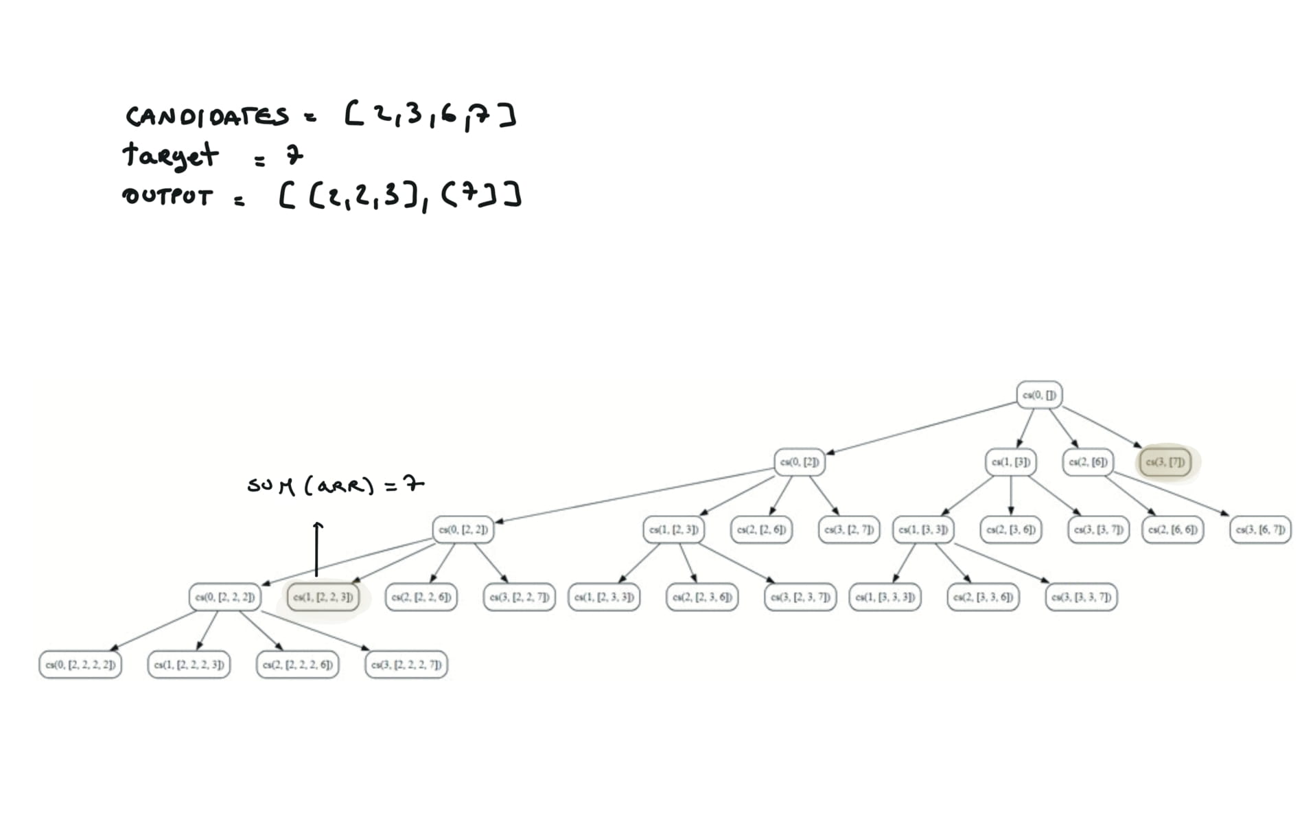
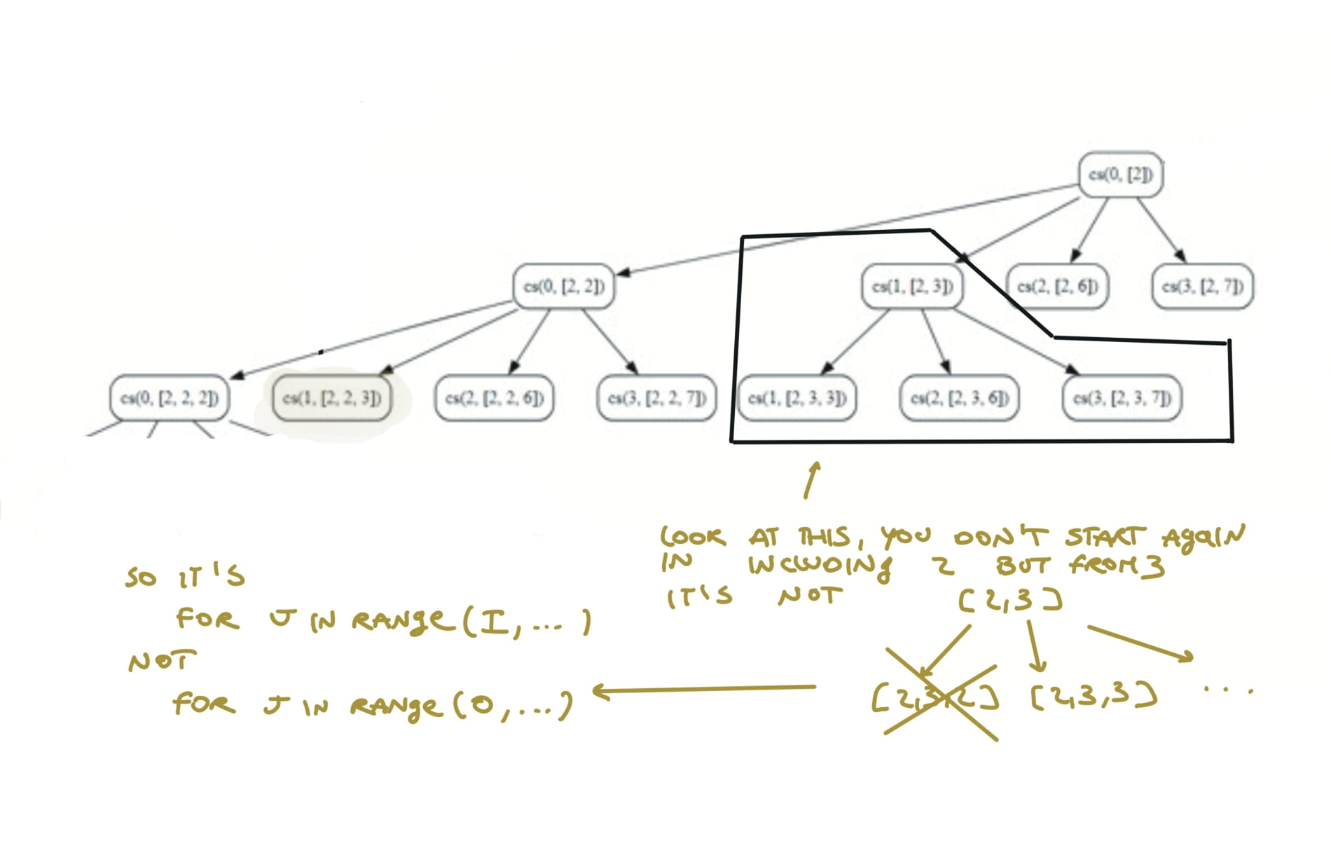
39. Combination Sum
[desc]
(link)
res = []
def dfs(i,sa):
    if sum(sa) == target:
        res.append(sa.copy())
        return
    if sum(sa) > target:
        return
    for j in range(i,len(candidates)):
		sa.append(candidates[j])
        dfs(j,sa)
		sa.pop()
dfs(0,[])
return res
visualization
90. Subsets II
[desc]
(link)
res = []
sub = []
nums.sort()
def backtrack(i):
    if i == len(nums):
        res.append(sub.copy())
        return
    sub.append(nums[i])
    backtrack(i+1)
    sub.pop()
    while i + 1 < len(nums) and nums[i] == nums[i + 1]:
        i += 1
    backtrack(i+1)
backtrack(0)
return res
Dynamic Programming
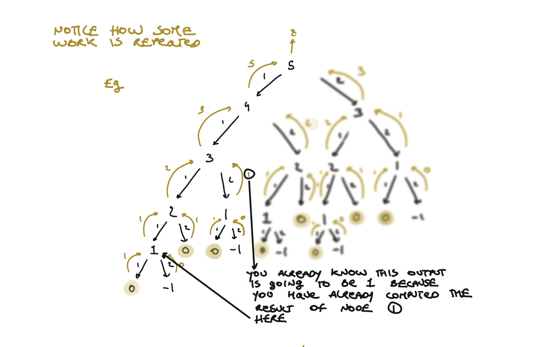
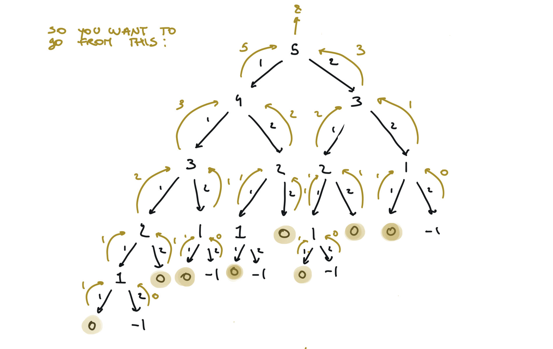
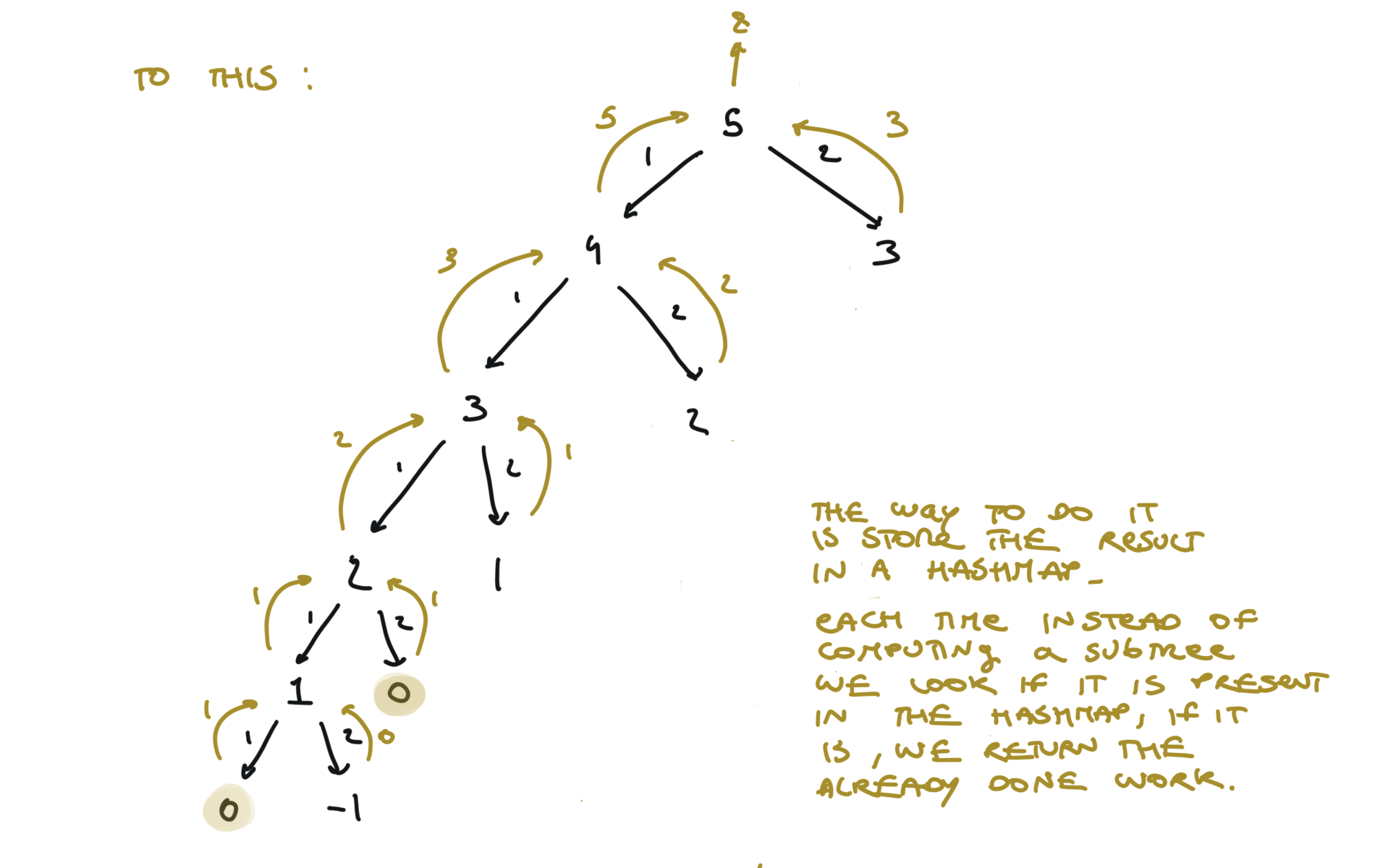
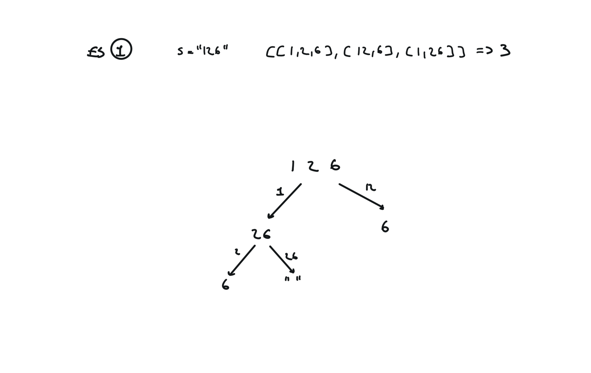
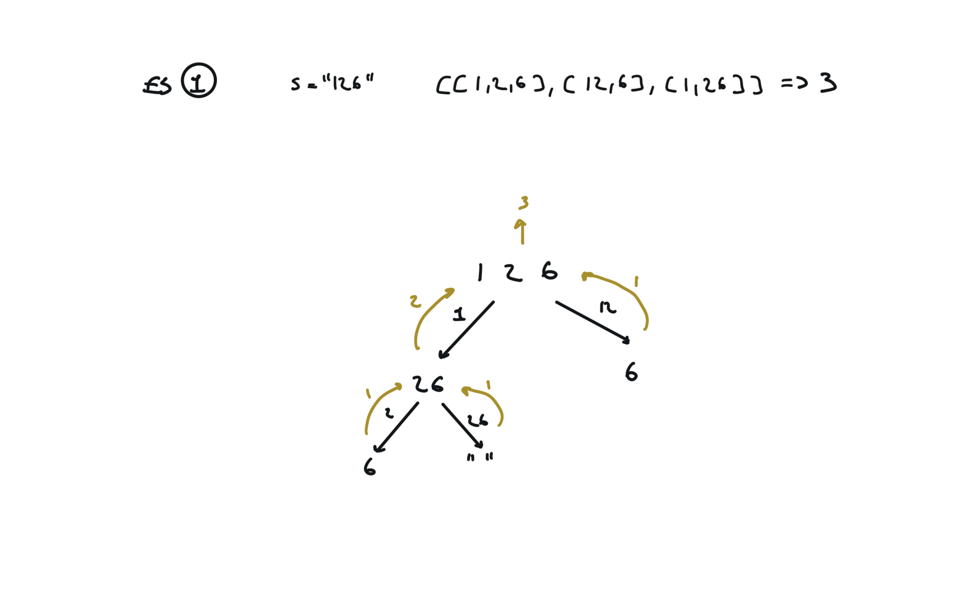
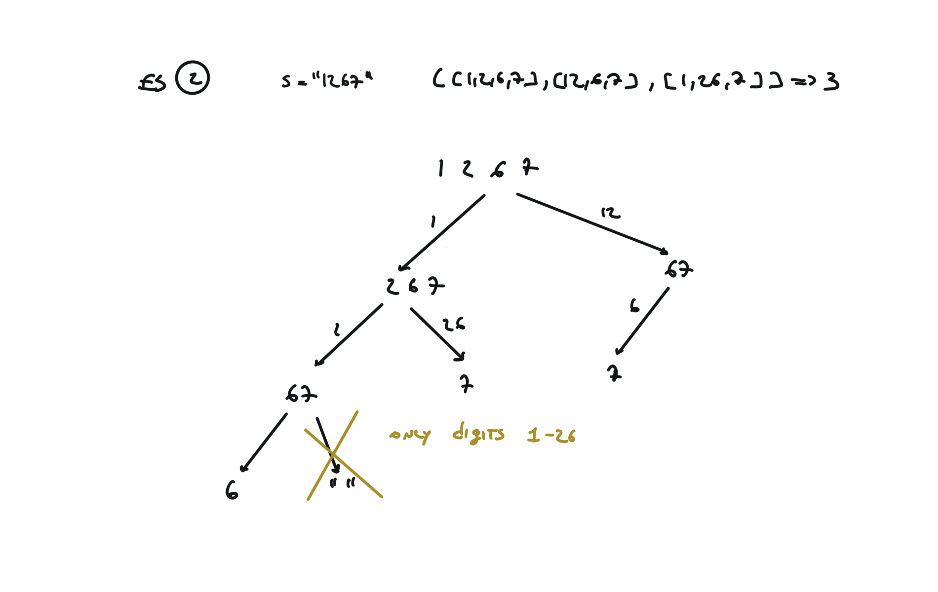
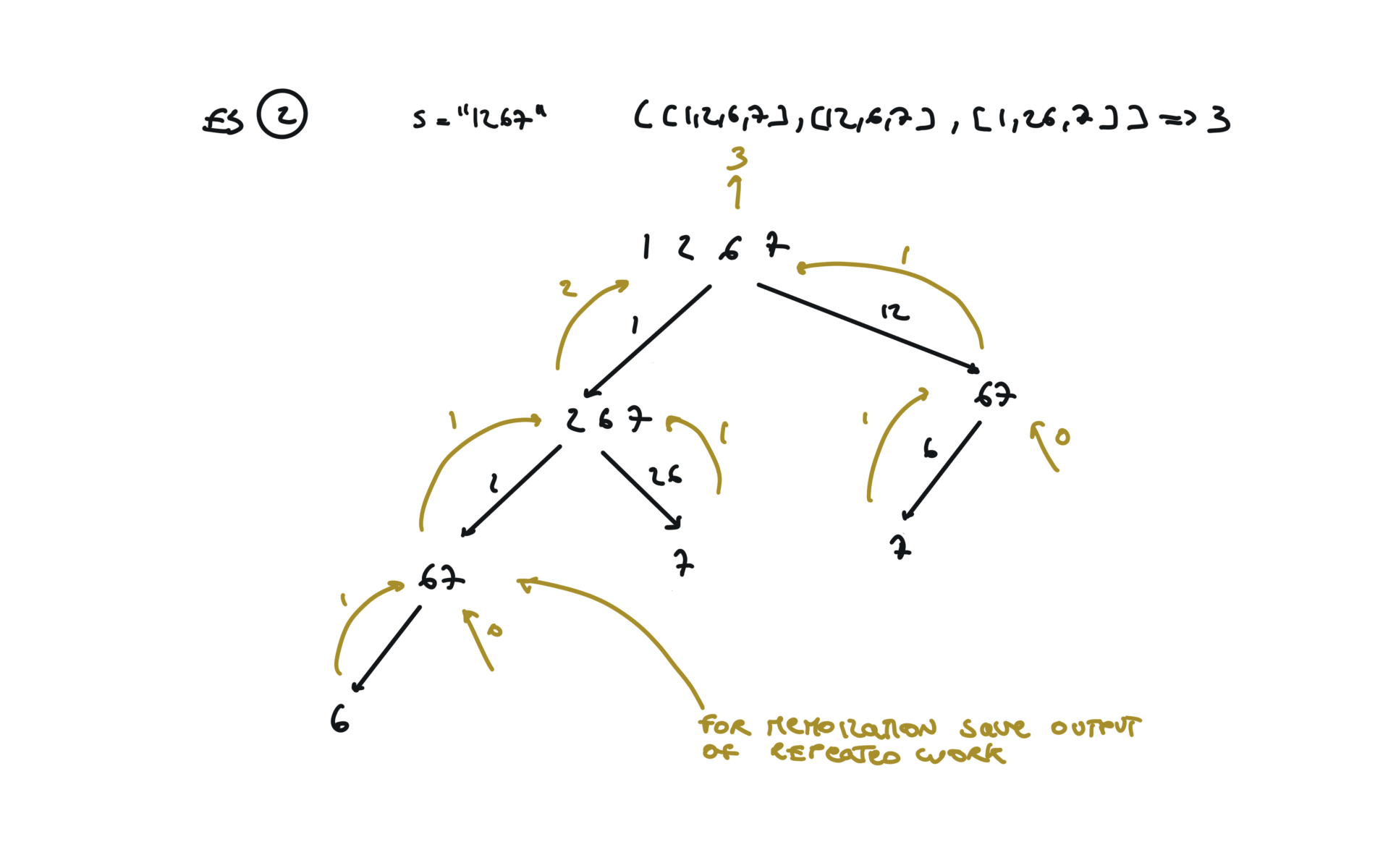
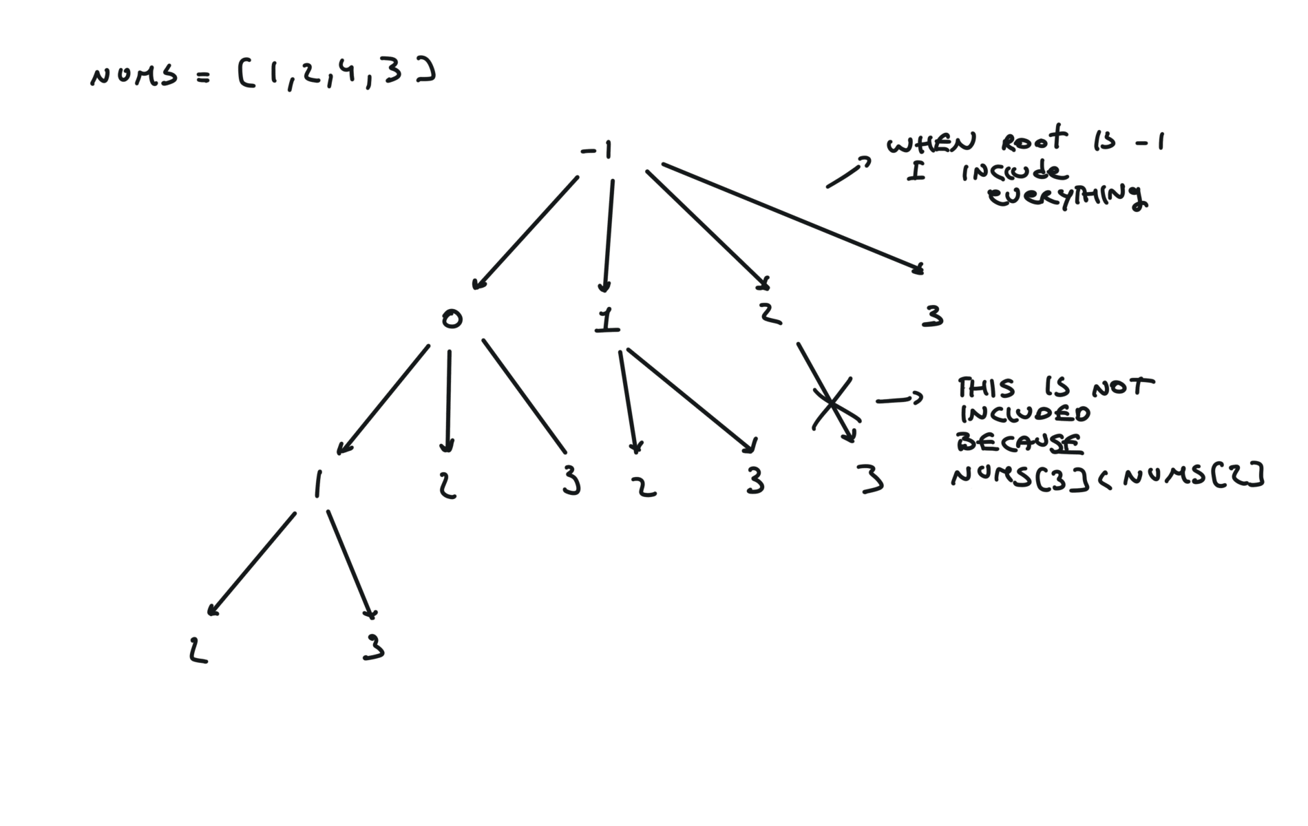
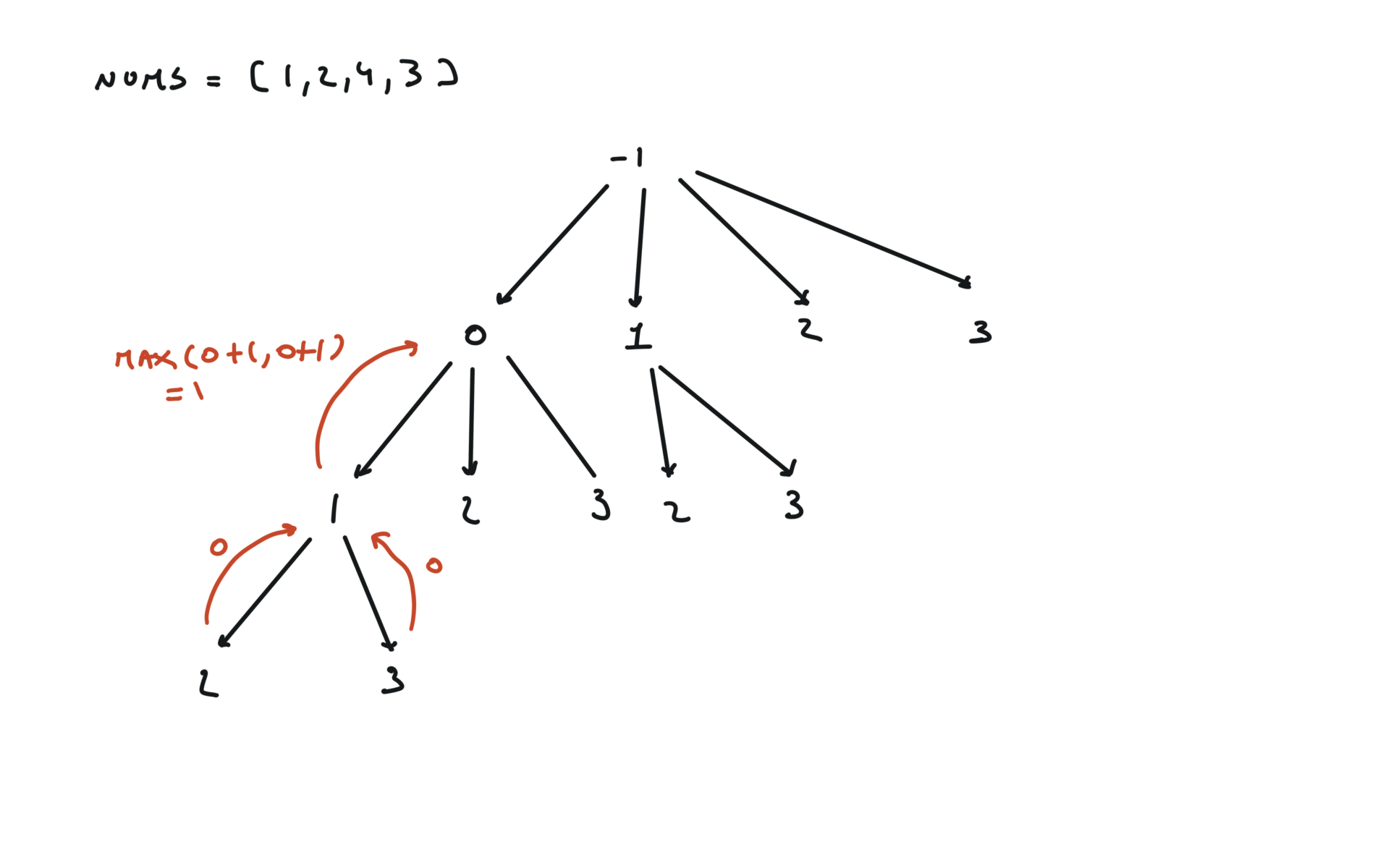
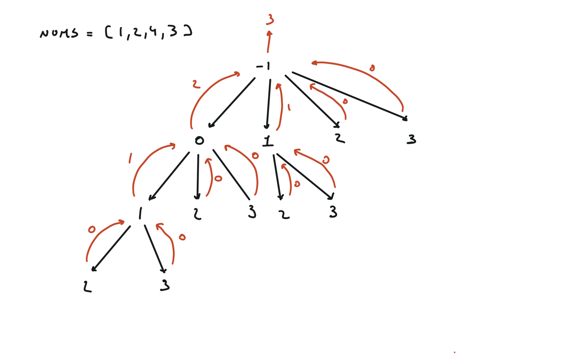
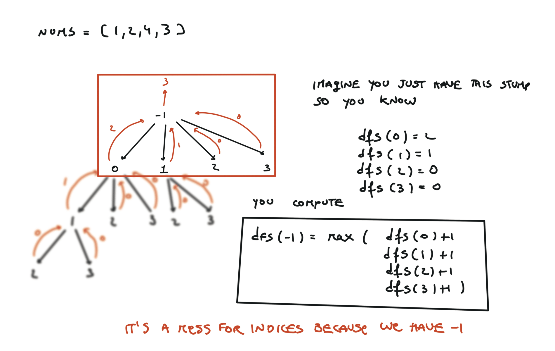
It is important, in order to easier the next step (memoization) that each node returns a value.
For example you can do a code that works but recursive calls does not return any value, like this: But it will be difficult now to achive the momoization step, what do we save into the dictionary? Here the node does not make any work, so we can’t save it’s work. Space complexity:
$$S(n) = O(n)$$
It is the depth of the recursion stack at max, which is $n$. Or look at the tree with this link
Space complexity:
$$S(n) = O(n)$$
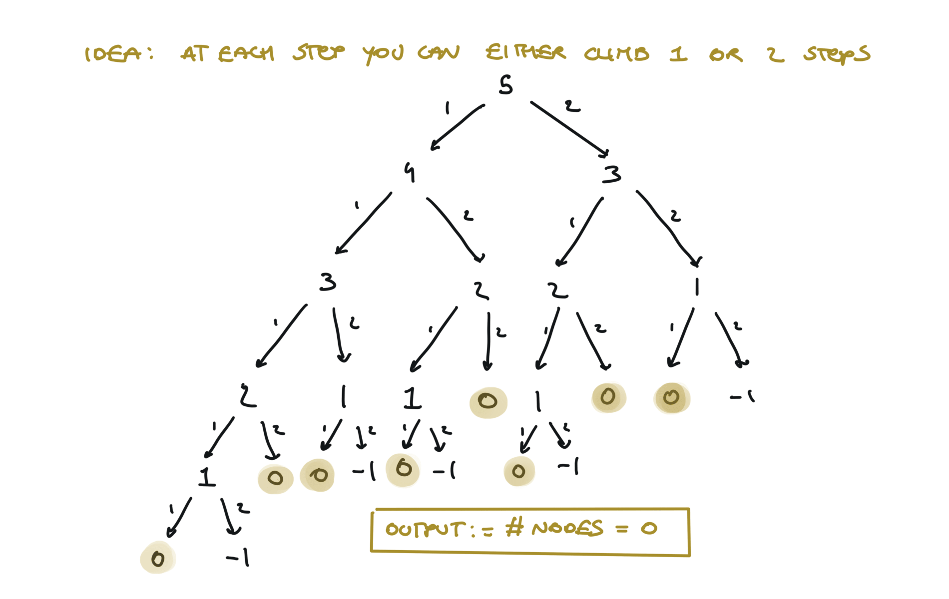
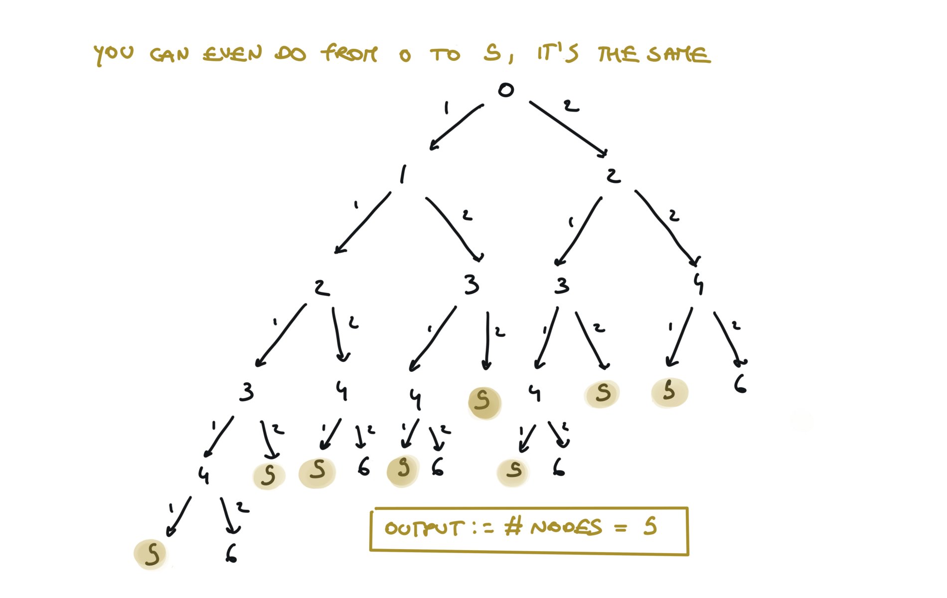
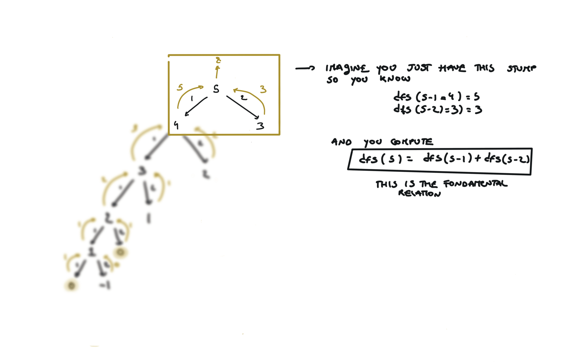
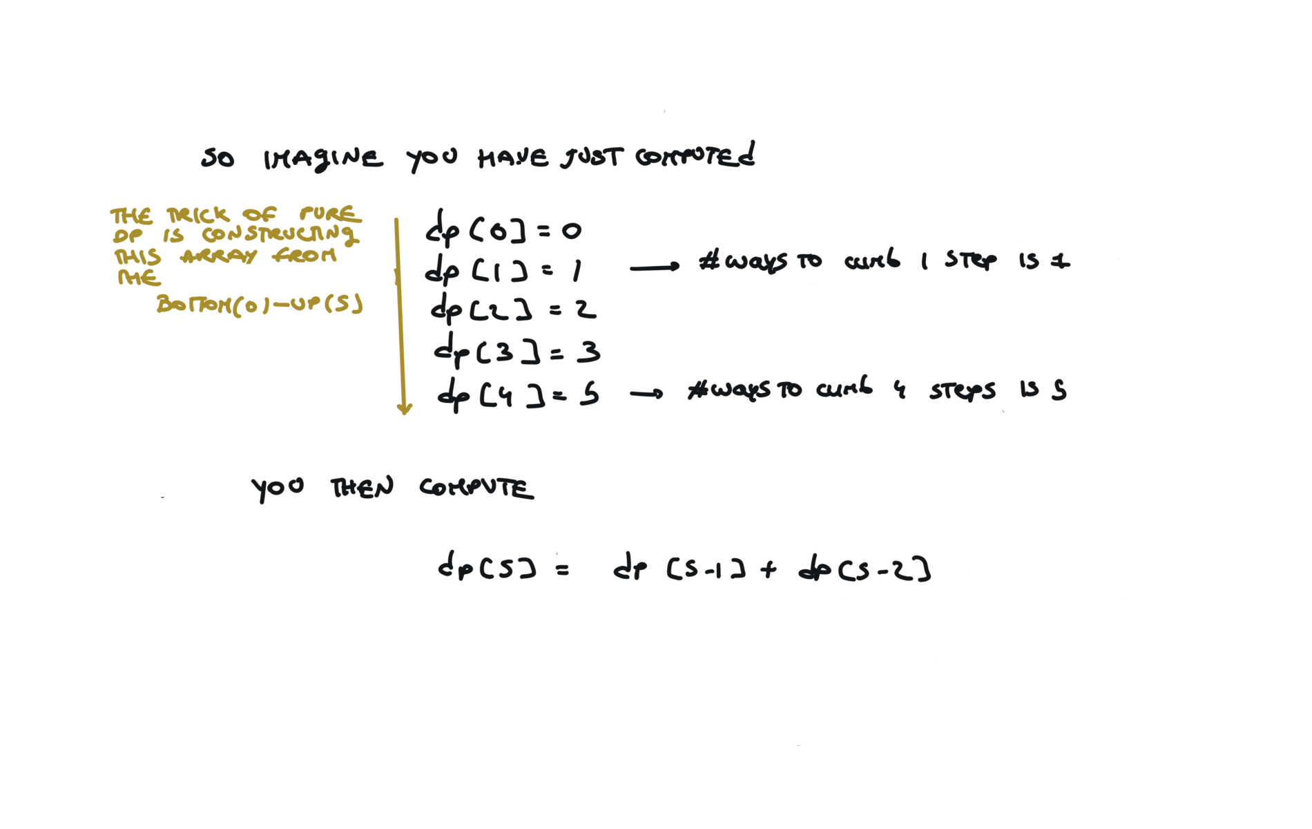
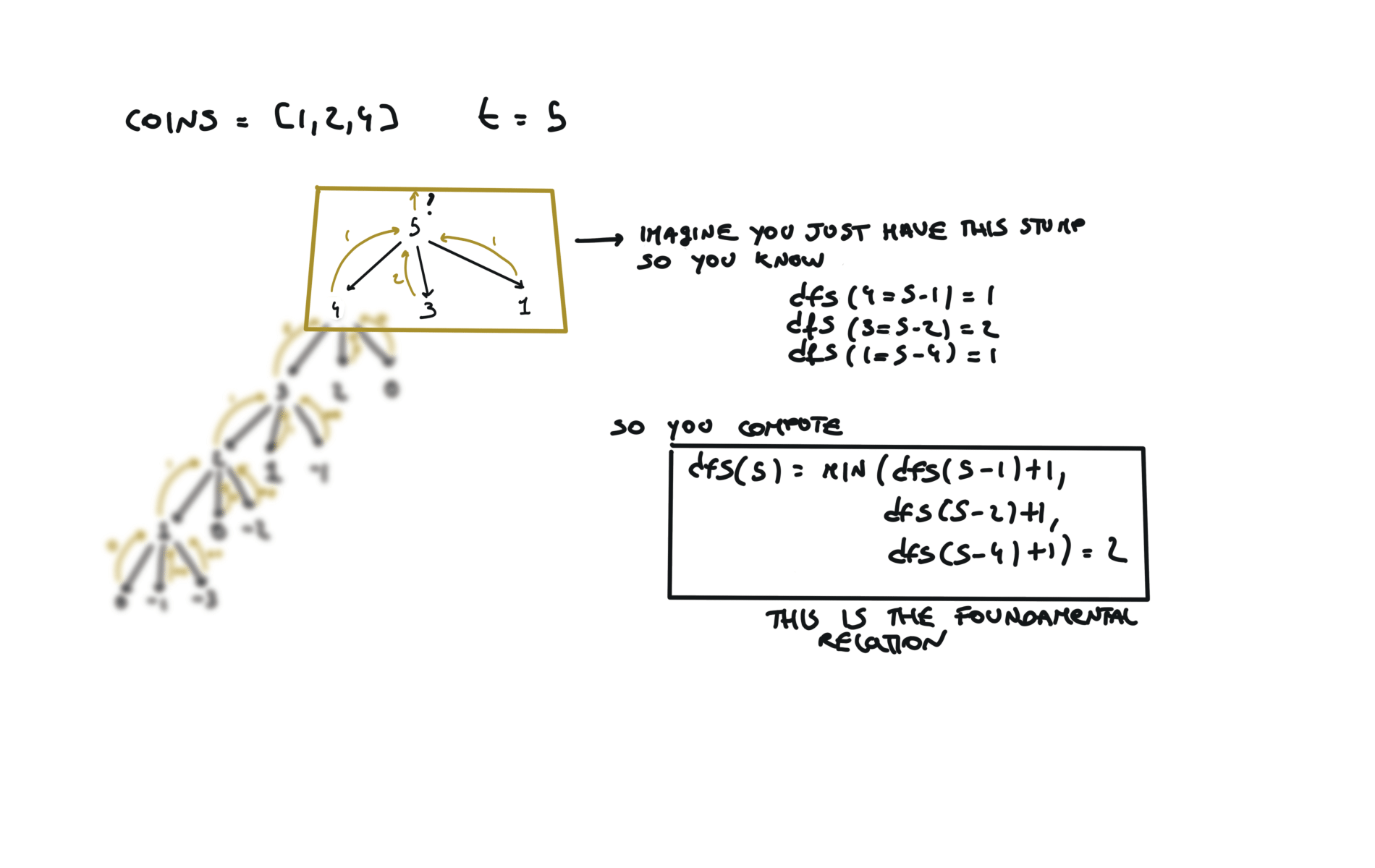
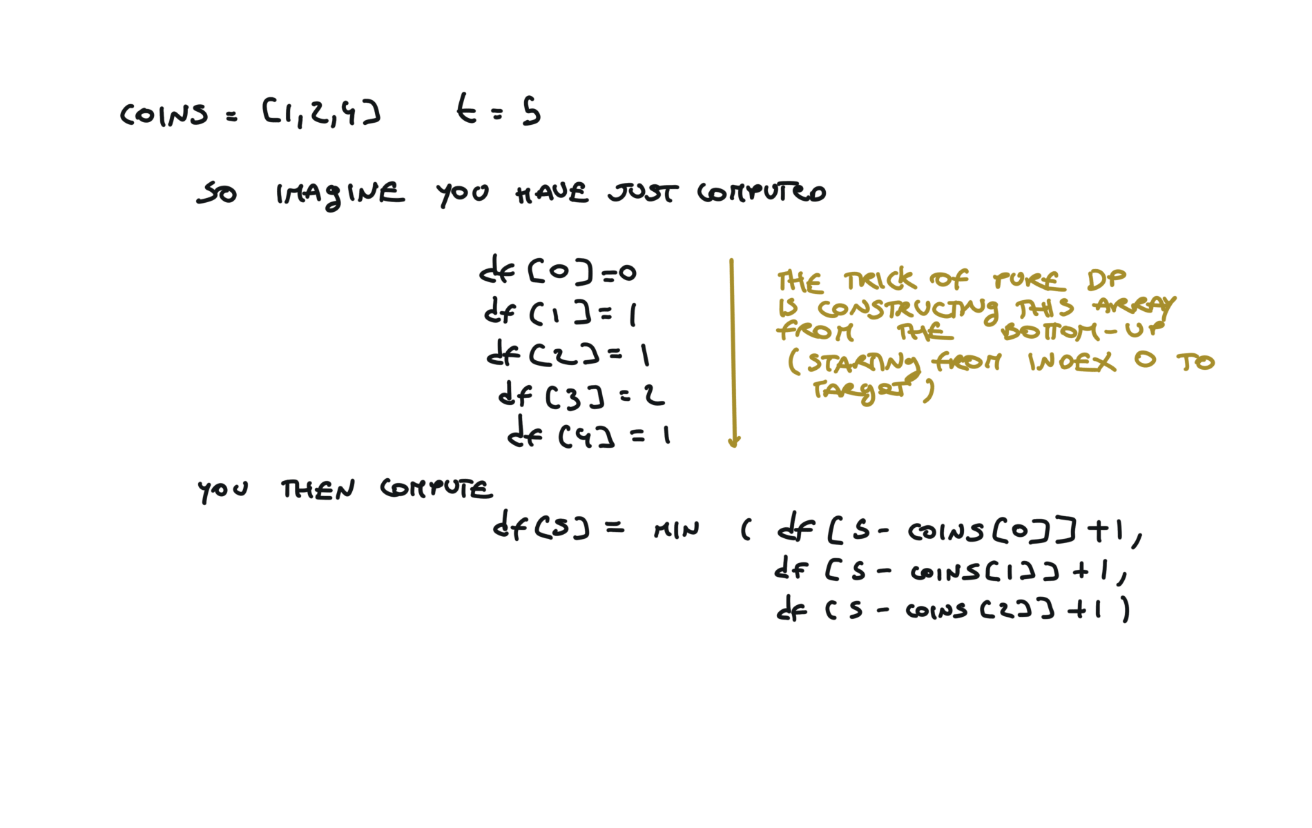
It is the depth of the recursion stack at max, which is $n$. The key to understand true dynamic programming is that we don’t ask the question: i’m at the 5th step, what are the ways i can reach this step? But you ask, progressively: i’m at the 5th step, what are the ways i can reach this step, given that i know how to reach each step below? Now it is easier, because, to reach the 5th step, you can take 1 step from 4th step or 2 step from step 3 and you already know in how many ways you can reach both of them. Space complexity:
$$S(n) = O(n)$$
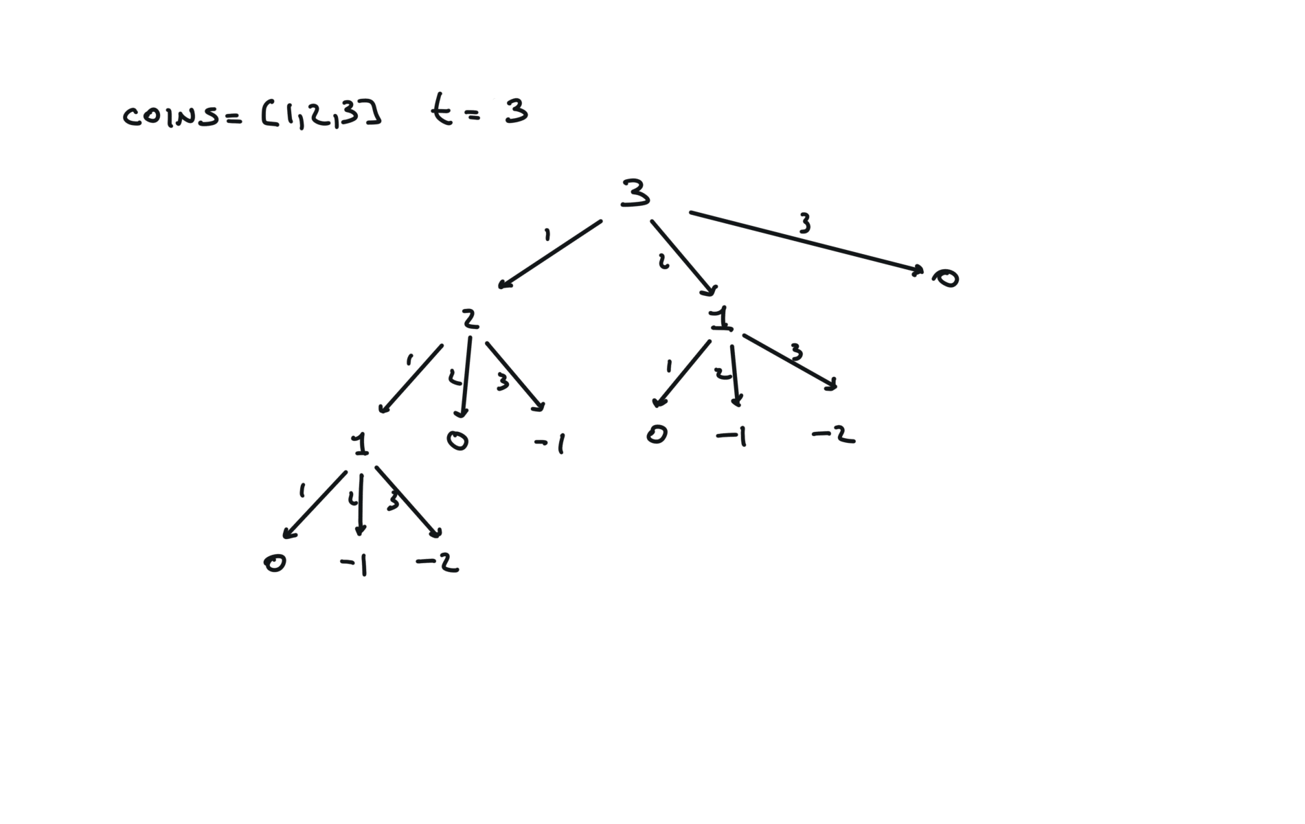
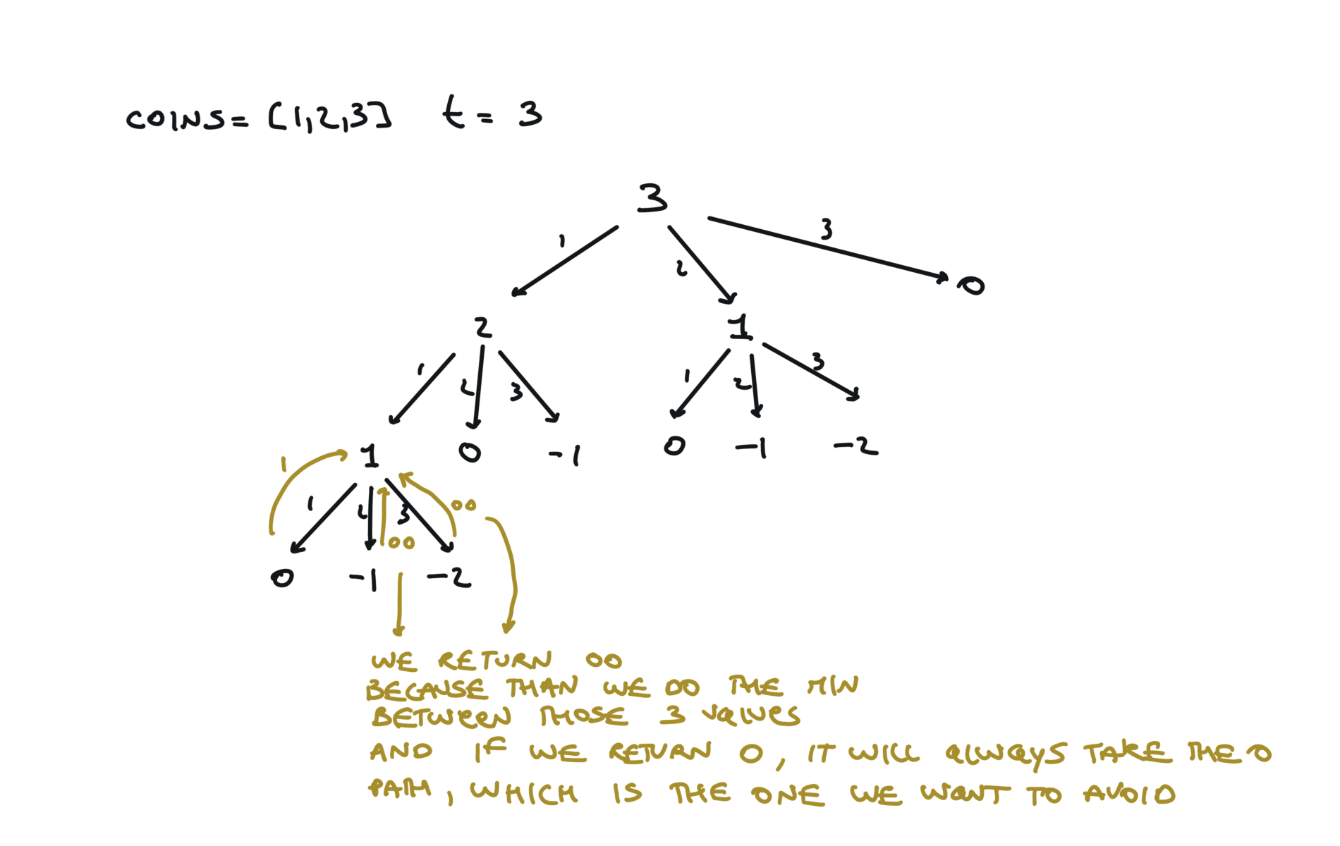
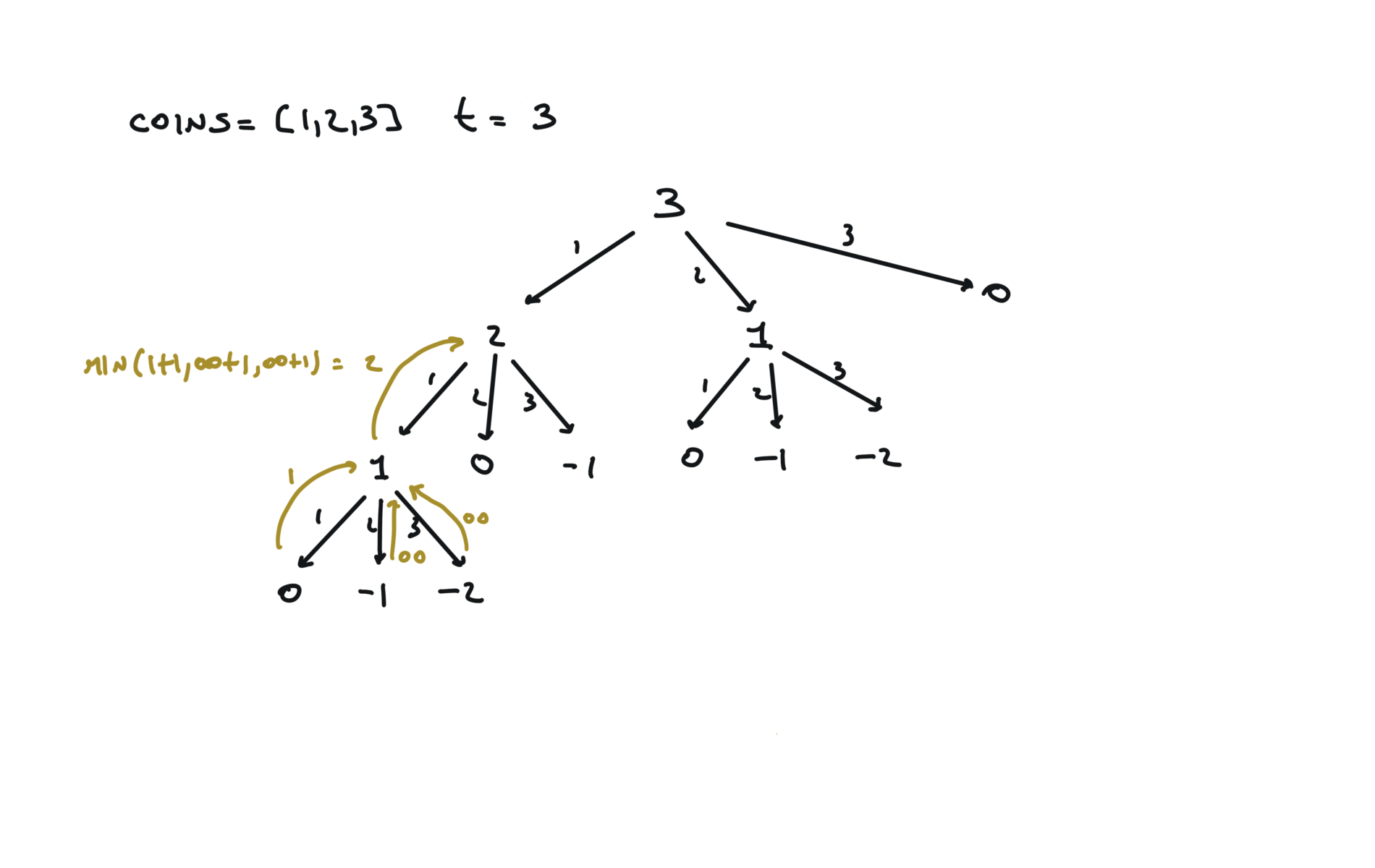
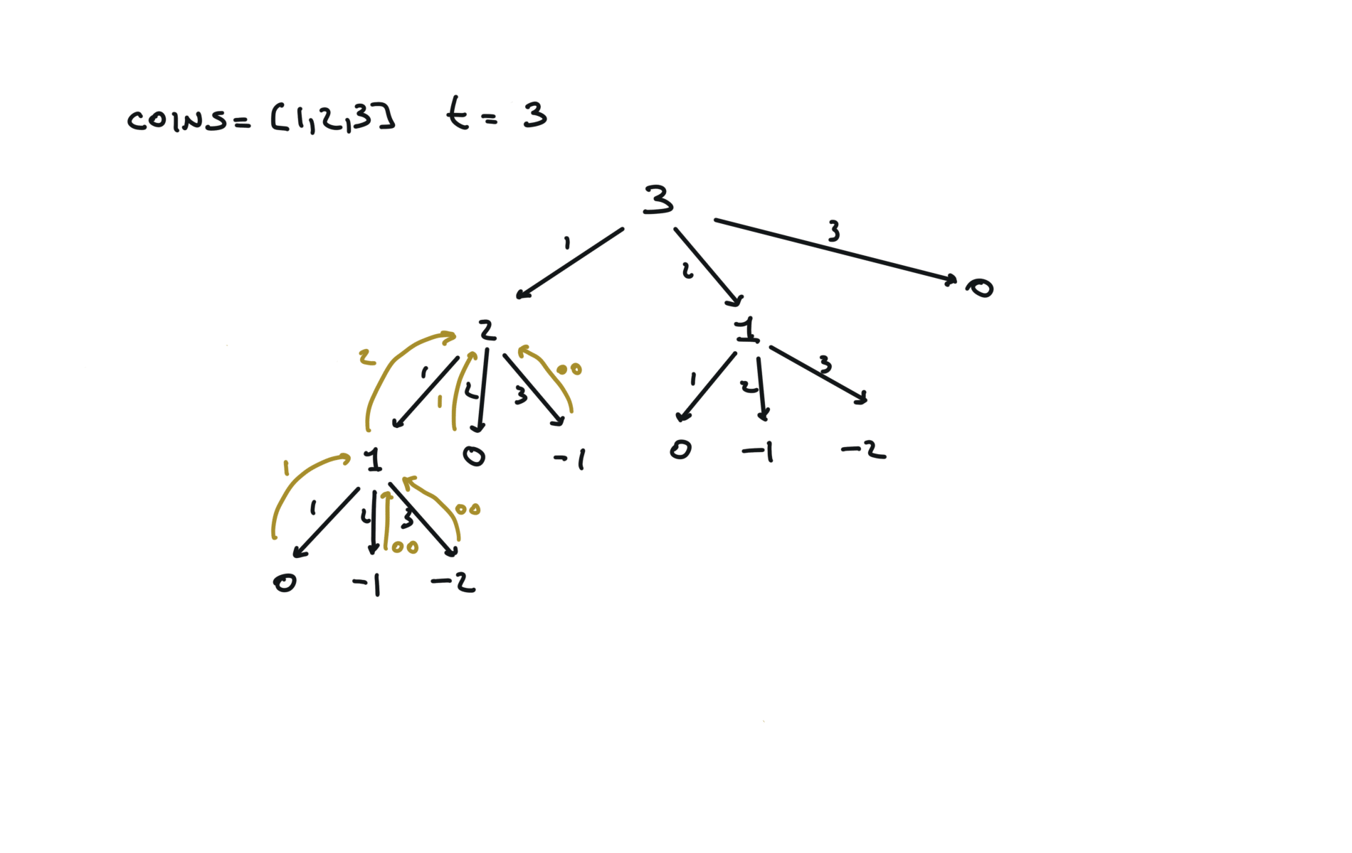
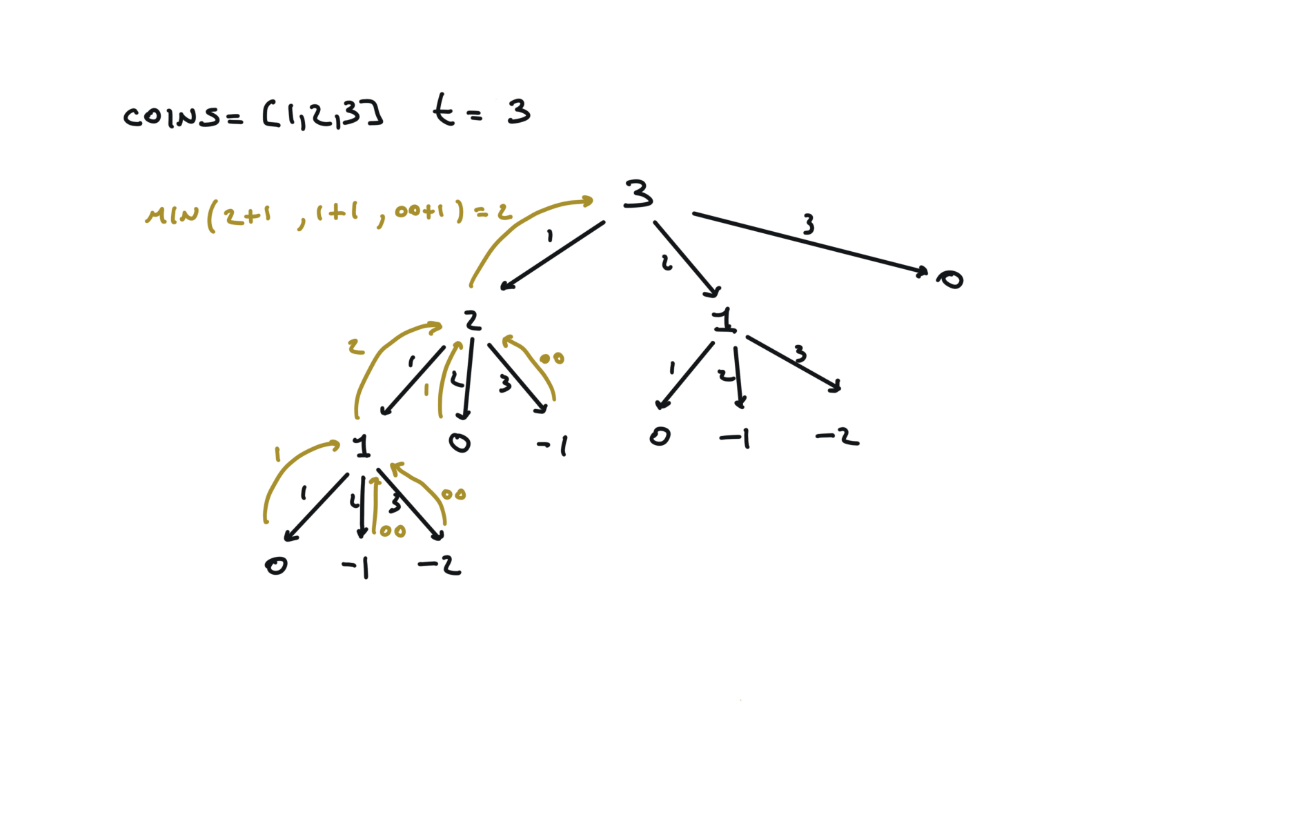
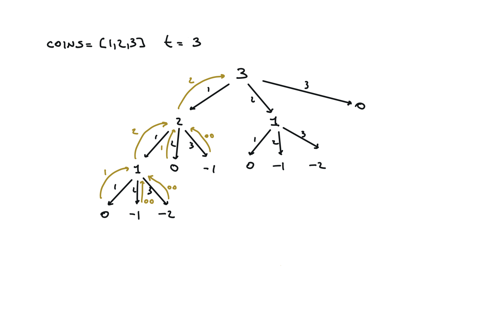
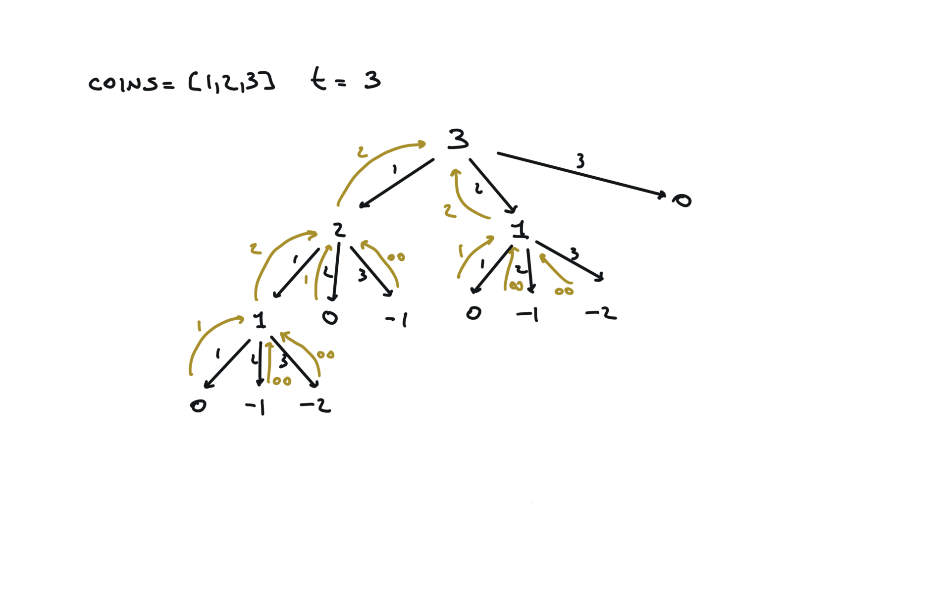
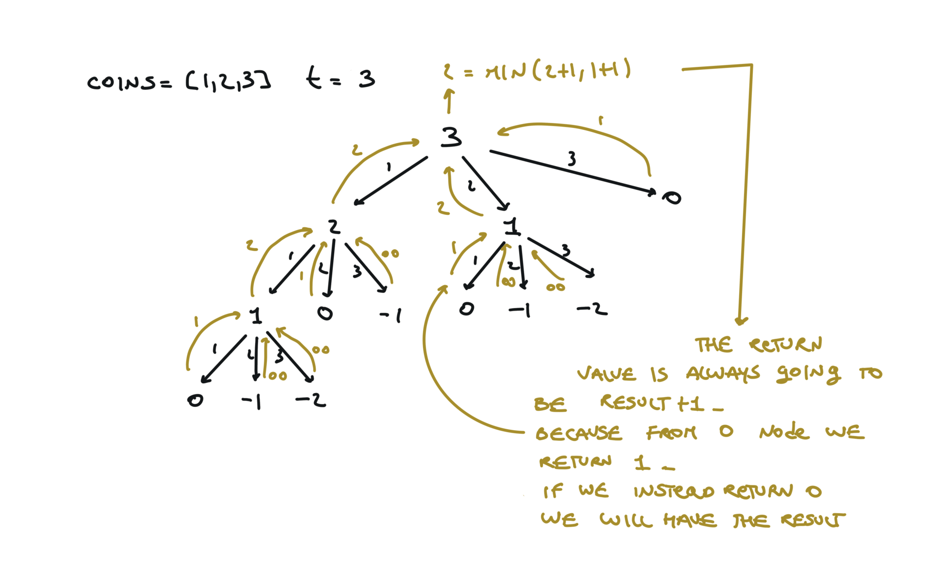
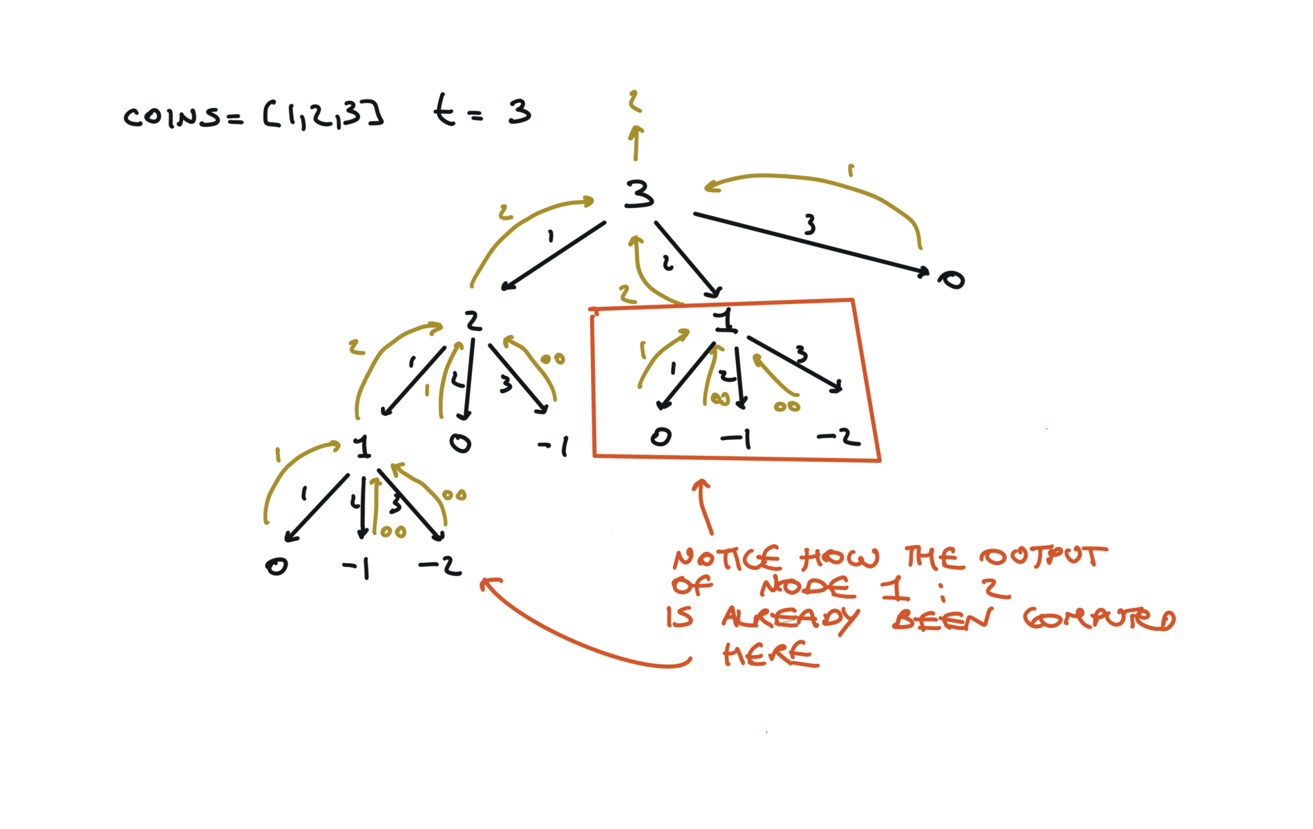
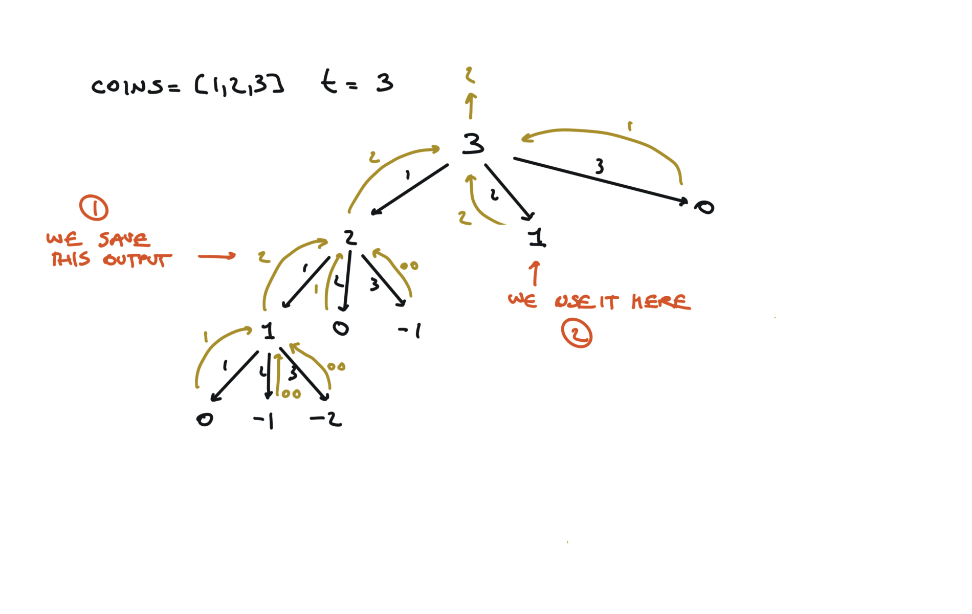
In the worst case we have in the available coins, a coin with value $1$. In this case the total amount is each time decreased by $1$. Space complexity:
$$S(n) = O(t)$$
It is the depth of the recursion stack at max, which is $t$. Space complexity:
$$S(n) = O(t)$$
It is the depth of the recursion stack at max, which is $t$. Space complexity:
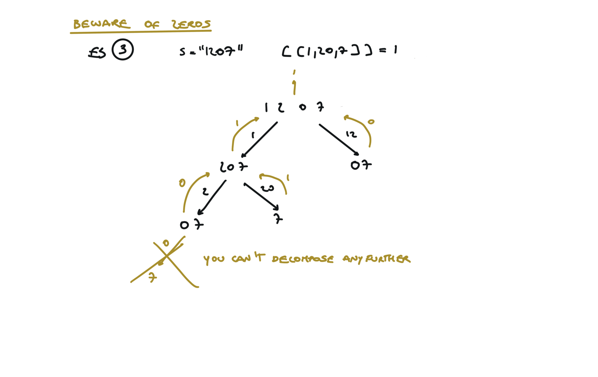
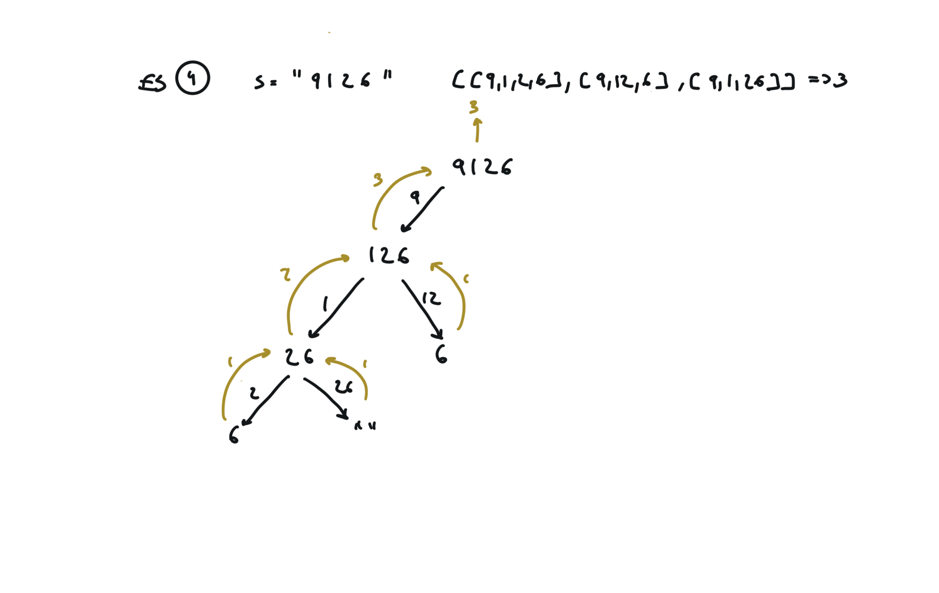
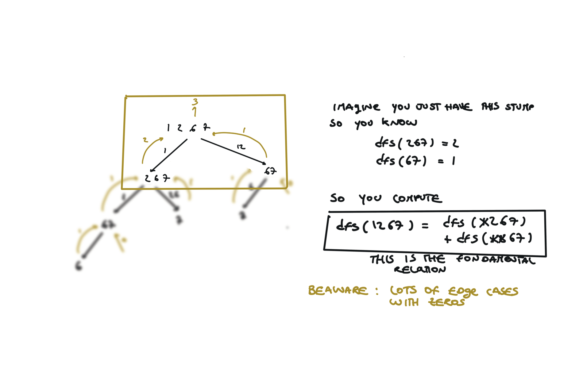
$$S(n) = O(t)$$ In this case i strongly believe the memoization solution is better and easier because you don’t have to handle a lot of edge cases involving zeros. Anyway here is the true dp solution.70. Climbing Stairs
[desc]
(link)
Naive DFS approach (TLE)
def dfs(step):
	if step == 0:
		return 1
	if step < 0:
		return 0
	l = dfs(step - 1)
	r = dfs(step - 2)
	return l + r
return dfs(n)
res = []
def dfs(step):
	if step == 0:
		res[0] += 1
		return
	if step < 0:
		return
	dfs(step - 1)
	dfs(step - 2)
return dfs(n)
visualization
time and space complexity
Dynamic Programming top-down (memoization)
mem = {}
def dfs(step):
	if step in mem:
		return mem[step]
	if step == 0:
		return 1
	if step < 0:
		return 0
	l = dfs(step - 1)
	r = dfs(step - 2)
	mem[step] = l + r
	return l + r
return dfs(n)
visualization
time and space complexity
Dynamic Programming bottom-up (true dynamic programming)
df = [1] * (n+1)
for i in range(2,n + 1):
	df[i] = df[i-1] + df[i-2]
return df[n]
visualization
time and space complexity
322. Coin Change
[desc]
(link)
Naive
def dfs(total):
    if total == 0:
        return 0
    if total < 0:
        return math.inf
    min_steps = math.inf
    for coin in coins:
        steps = dfs(total + coin)
        min_steps = min(min_steps, steps + 1)
    return min_steps
result = dfs(amount)
return result if result != math.inf else -1
visualization
time and space complexity
Top-Down (memoization)
memo = {}
def dfs(total):
    if total in memo:
        return memo[total]
    if total == 0:
        return 0
    if total < 0:
        return math.inf
    min_steps = math.inf
    for coin in coins:
        steps = dfs(total + coin)
        min_steps = min(min_steps, steps + 1)
    memo[total] = min_steps
    return min_steps
result = dfs(amount)
return result if result != math.inf else -1
visualization
time and space complexity
bottom-up (true dp)
dp = [amount + 1] * (amount + 1)
dp[0] = 0
for a in range(1, amount + 1):
    for c in coins:
        if a - c >= 0:
            dp[a] = min(dp[a], 1 + dp[a - c])
return dp[amount] if dp[amount] != amount + 1 else -1
visualization
time and space complexity
91. Decode Ways
[desc]
(link)
Top-Down (memoization)
memo = {}
def dfs(s):
    if s in memo:
		return memo[s]
    if len(s) == 0 or (len(s) == 1 and int(s) != 0):
        return 1
    l, r = 0, 0
    if int(s[0]) > 0:
        l = dfs(s[1:])
    if int(s[0:2]) > 9 and int(s[0:2]) < 27:
        r = dfs(s[2:])
    memo[s] = l + r
    return l + r
return dfs(s)
visualization
bottom-up
dp = {}
dp[""] = 1
for i in range(len(s)-1,-1,-1):
    sub = s[i:len(s)]
    if int(sub[0]) > 0:
        dp[sub] = dp[sub[1:]]
    else:
        dp[sub] = 0
    if len(sub) > 1 and 9 < int(sub[0:2]) < 27:
        dp[sub] += dp[sub[2:]]
return dp[s]
visualization
55. Jump Game
[desc]
(link)
DFS with memoization
cache = {}
def dfs(i):
    if i in cache:
        return cache[i]
    if i == len(nums) - 1:
        return True
    tmp = False
    for j in range(nums[i]):
        tmp = tmp or dfs(j+1+i)
    cache[i] = tmp
    return tmp
return dfs(0)
true dp
n = len(nums)
dp = [False] * n
dp[n - 1] = True
for i in range(n-2,-1,-1):
    found = False
    j = 1
    while j <= nums[i] and not found:
        if i+j < n and dp[i + j]:
			dp[i] = True
			found = True
        j+= 1
return dp[0]
greedy solution
goal = len(nums)-1
for i in range(goal-1,-1,-1):
    if i+nums[i] >= goal:
        goal = i
return goal == 0
45. Jump Game II
[desc]
(link)
DFS with memoization
cache = {}
def dfs(i):
    if i in cache:
        return cache[i]
    if i >= len(nums) - 1:
        return 0
    minn = math.inf
    for j in range(nums[i]):
        minn = min(minn, dfs(j+1+i) + 1)
    cache[i] = minn
    return minn
return dfs(0)
true dp
n = len(nums)
dp = [0] * n
dp[n - 1] = 0
for i in range(n-2,-1,-1):
    minn = math.inf
    j = 1
    while j <= nums[i]:
        if i + j < n:
            minn = min(dp[i+j]+1,minn)
        j+= 1
    dp[i] = minn
return dp[0]
300. Longest Increasing Subsequence
[desc]
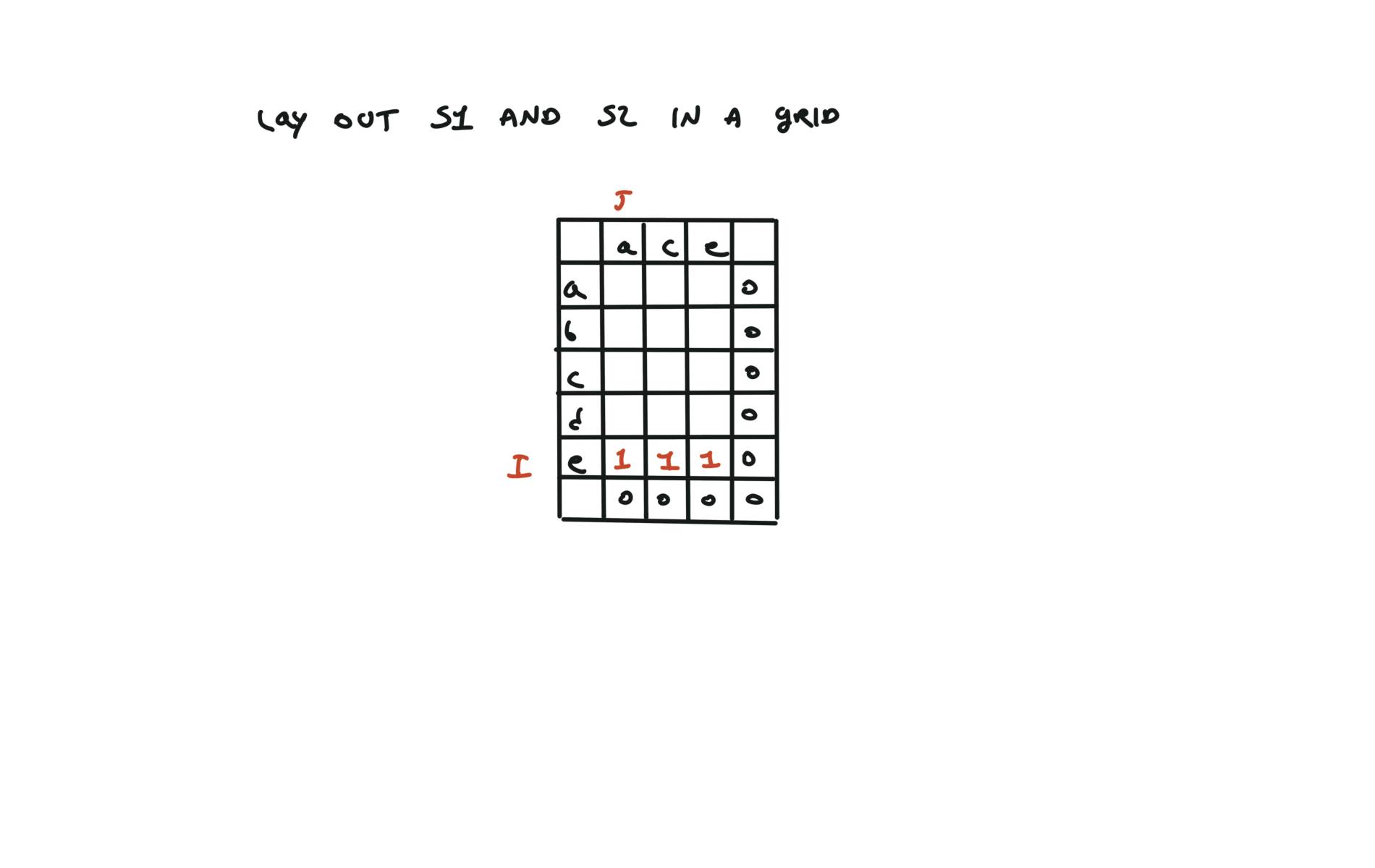
(link)
top-down (memoization)
memo = {}
def dfs(i):
	if i == len(nums):
		return 0
	if i in memo:
		return memo[i]
	a = 0
	for j in range(i+1,len(nums)):
		if i == -1 or nums[j] > nums[i]:
			a = max(a, dfs(j) + 1)
    memo[i] = a
	return a
return dfs(-1)
visualization
bottom-up
n = len(nums)
LIS = [0] * (n+1)
for i in range(n-1,-1,-1):
	a = 0
	for j in range(i+1,n+1):
		a = max(a, LIS[j] + 1 if nums[i-1] < nums[j-1] or i == 0 else 0)
	LIS[i] = a
return LIS[0]
visualization
2D Dynamic Programming
1143. Longest Common Subsequence
[desc]
(link)
top-down
def dfs(i, j):
    if i == len(text1) or j == len(text2):
		return 0
	if text1[i] == text2[j]:
        return 1 + dfs(i + 1, j + 1)
	else:
		return max(dfs(i + 1, j), dfs(i, j + 1))
return dfs(0, 0)
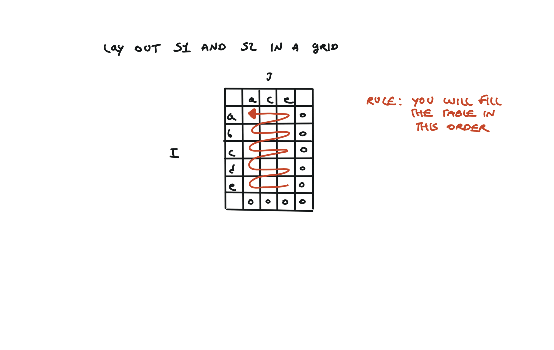
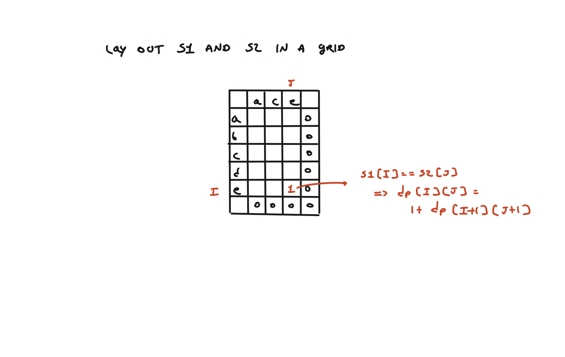
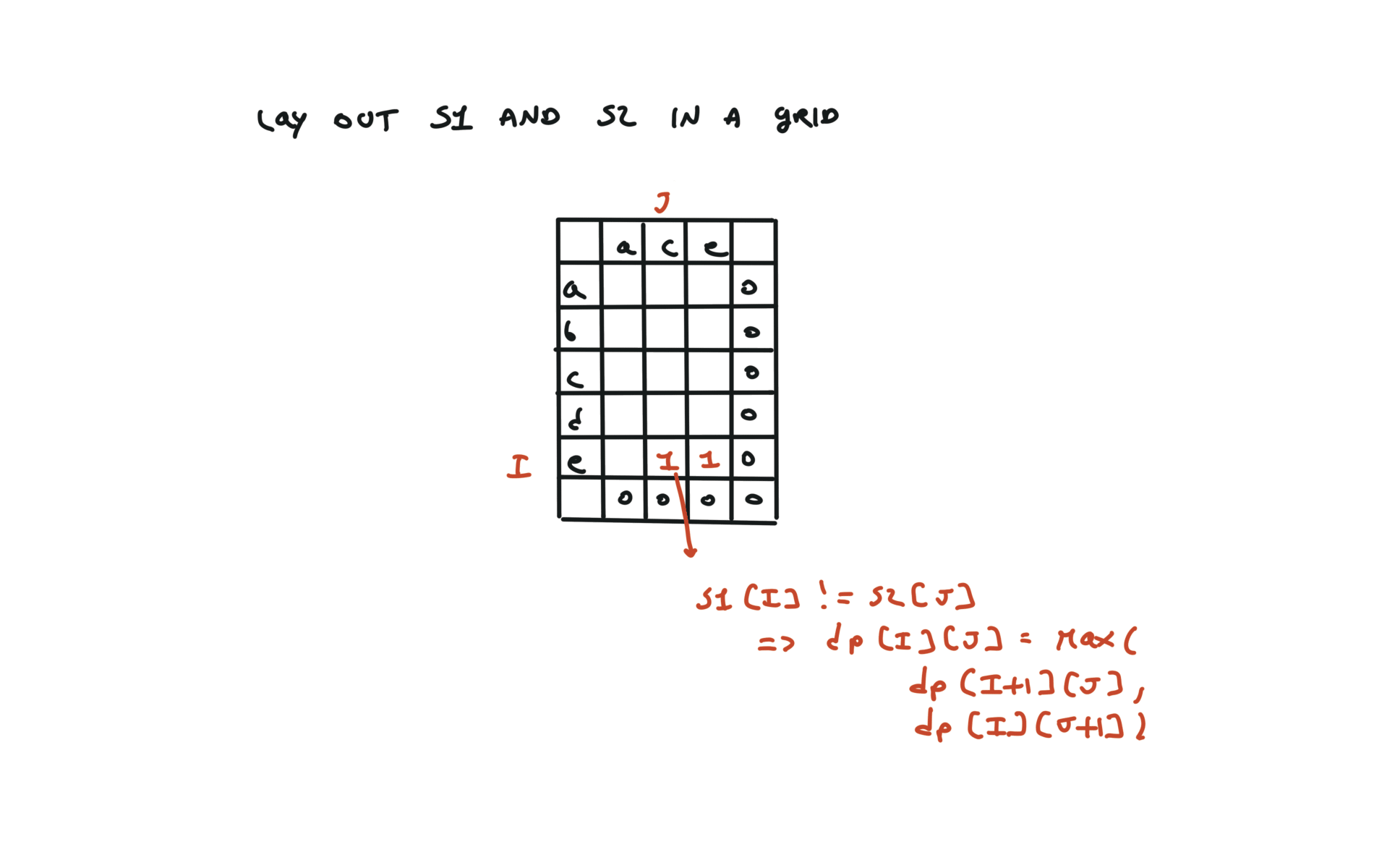
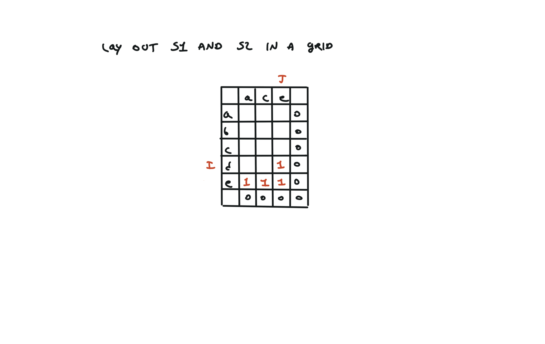
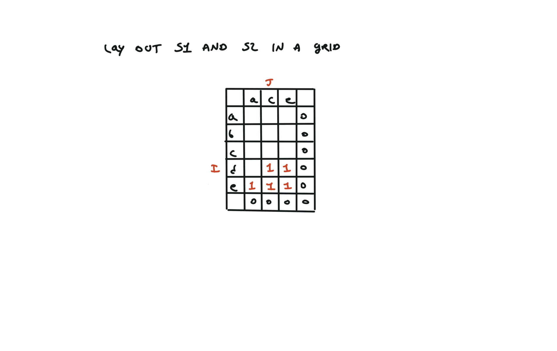
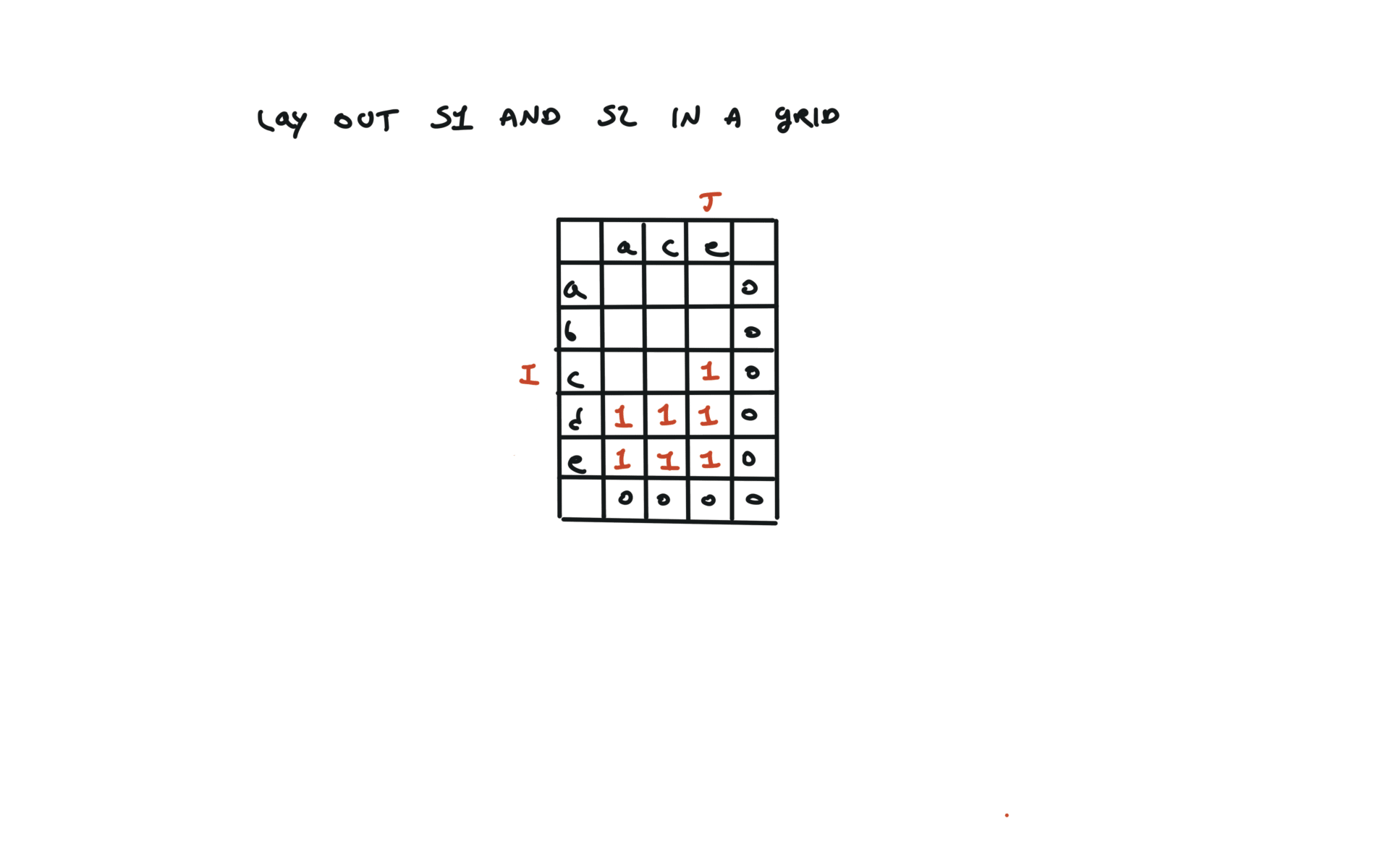
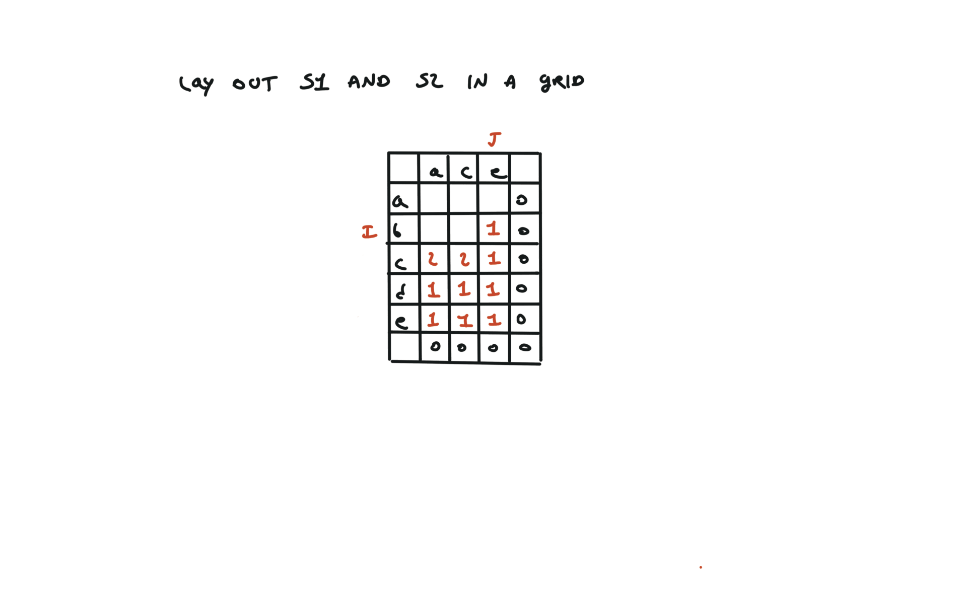
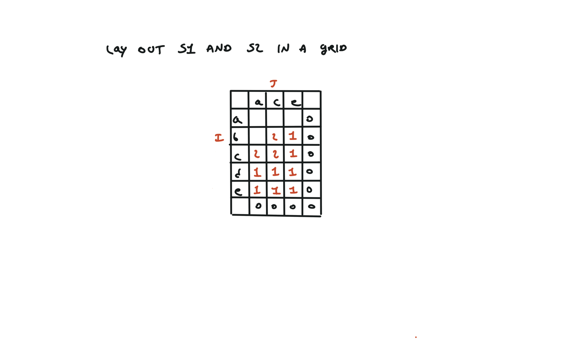
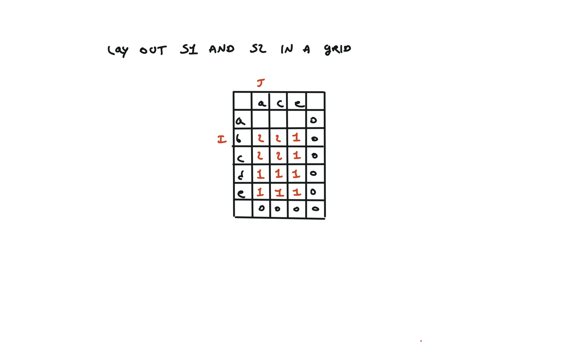
visualization
bottom-up
dp = [[0 for j in range(len(text2) + 1)]
	for i in range(len(text1) + 1)]
for i in range(len(text1) - 1, -1, -1):
	for j in range(len(text2) - 1, -1, -1):
		if text1[i] == text2[j]:
			dp[i][j] = 1 + dp[i + 1][j + 1]
		else:
			dp[i][j] = max(dp[i][j + 1], dp[i + 1][j])
return dp[0][0]
visualization
72. Edit Distance
[desc]
(link)
top-down
def dfs(i, j):
	if i == len(word1):
		return len(word2) - j
	if j == len(word2):
		return len(word1) - i
	if word1[i] == word2[j]:
		return dfs(i + 1, j + 1)
	else:
		return 1 + min(dfs(i, j + 1), dfs(i + 1, j), dfs(i + 1, j + 1))
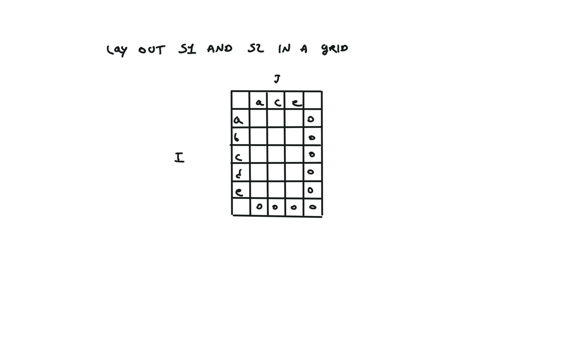
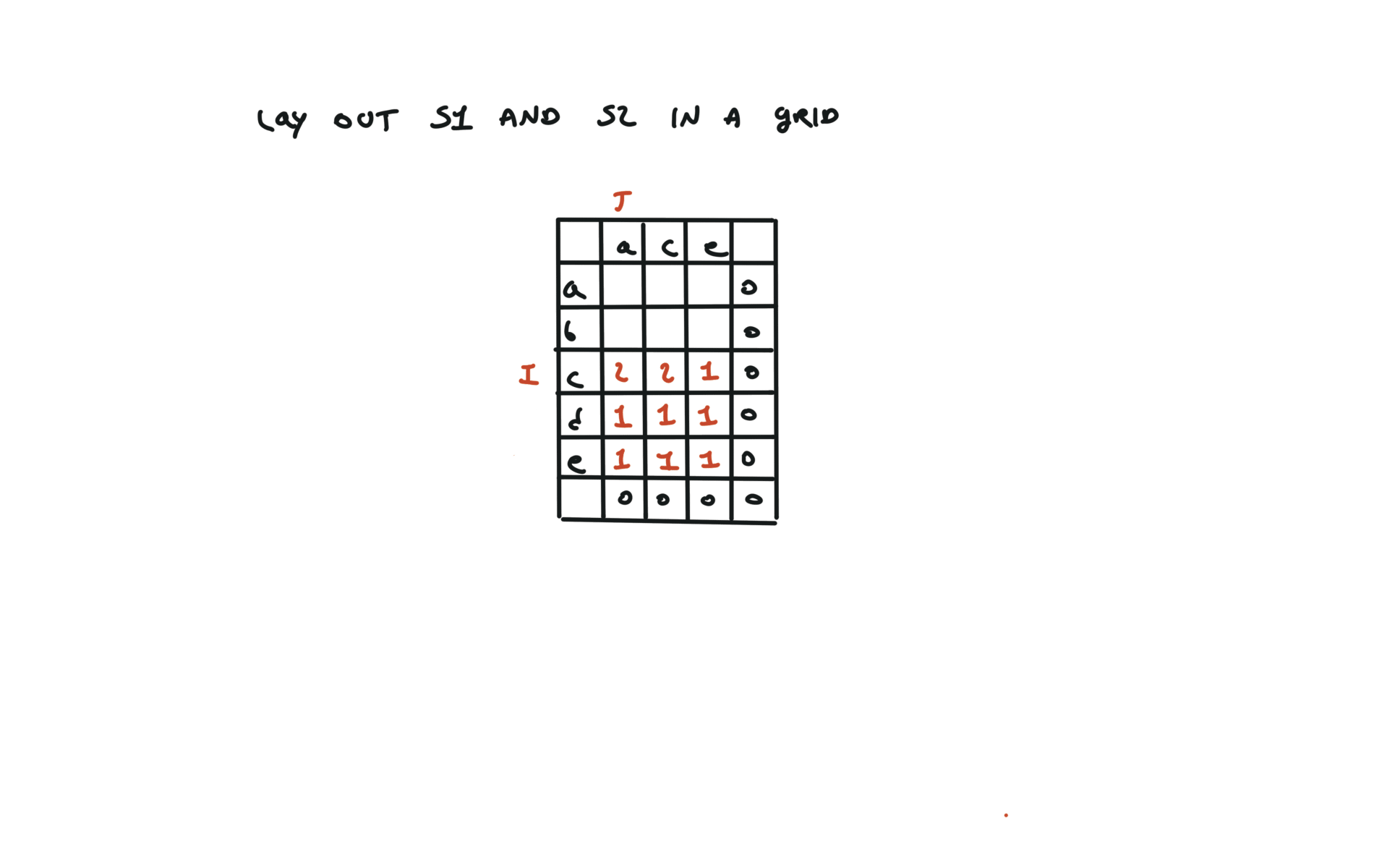
return dfs(0,0)
bottom-up
dp = [[0 for j in range(len(word2) + 1)]
	for i in range(len(word1) + 1)]
for i in range(len(word1) + 1):
	dp[i][len(word2)] = len(word1) - i
for j in range(len(word2) + 1):
	dp[len(word1)][j] = len(word2) - j

for i in range(len(word1) - 1, -1, -1):
	for j in range(len(word2) - 1, -1, -1):
		if word1[i] == word2[j]:
			dp[i][j] = dp[i+1][j+1]
		else:
			dp[i][j] = 1 + min(dp[i][j+1], dp[i+1][j], dp[i+1][j+1])
return dp[0][0]
Graphs
All graphs visits have the same complexity. $$ O( \sum_{v \in G} (1 + \tau(v))) = O( n + \sum_{v \in G} \tau(v))$$ Where $\tau(v)$ is the cost of the operation of getting incident edges for a given node $v$.
The cost of this operation depends on the graph representation. The space complexity is
$$S(n) = O(n + m)$$visits
BFS
def bfs(root):
	q = deque([root])
	mark root
	while q:
		u = q.popleft()
		for all edges(u,v):
			if v is not marked:
				mark v
				q.append(v)
DFS-recurisve
def dfs(u):
	mark u
	for all edges(u,v):
		if v is not marked:
			dfs(v)
DFS-iterative
def dfs(root):
	s = [root]
	mark root
	while s:
		u = s.pop()
		for all edges(u,v):
			if v is not marked:
				mark v
				s.append(v)
time and space complexity
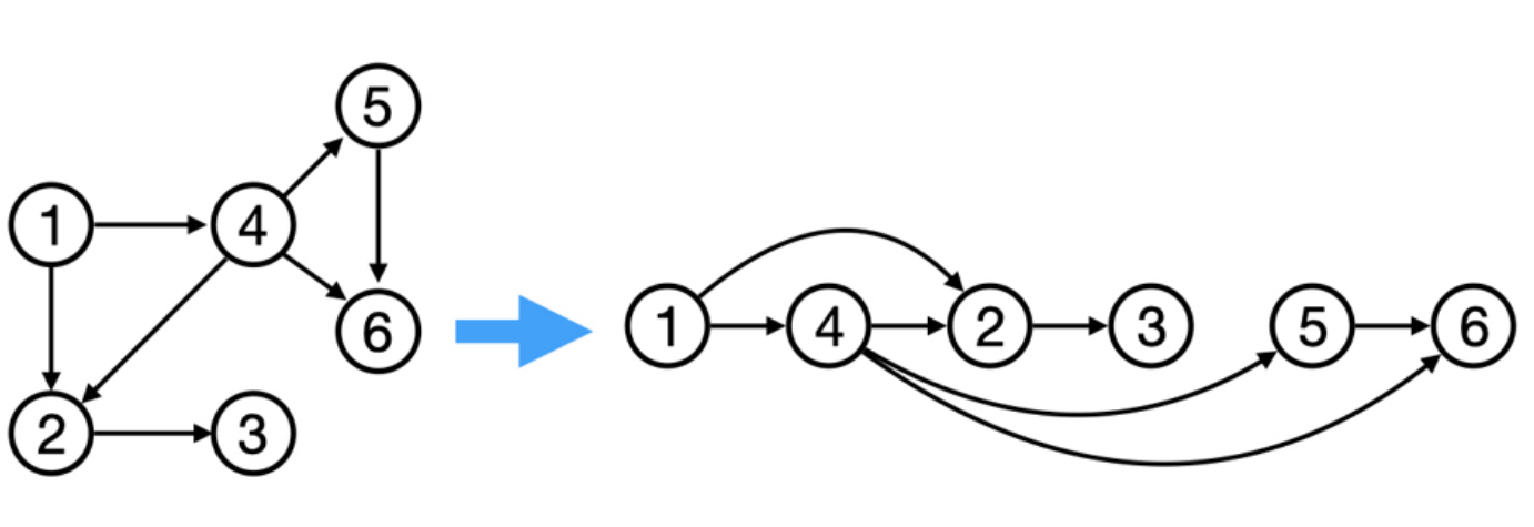
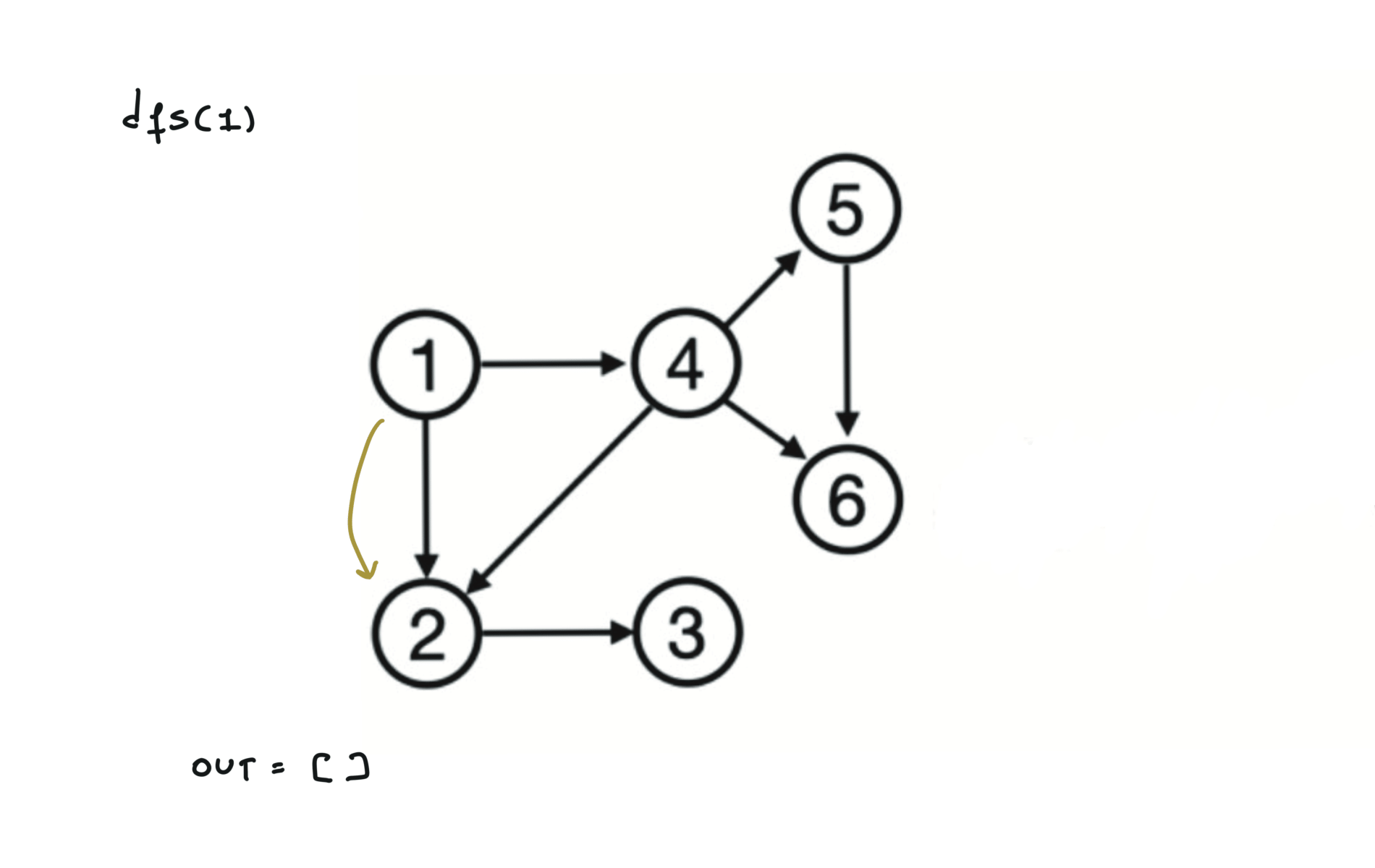
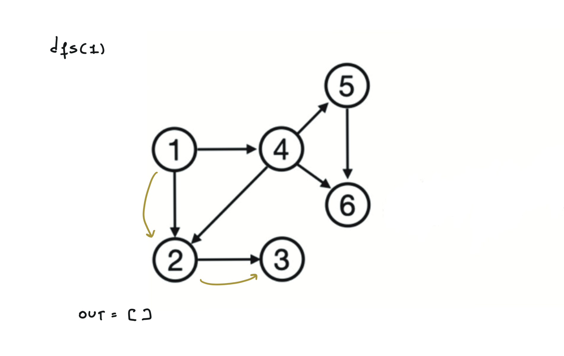
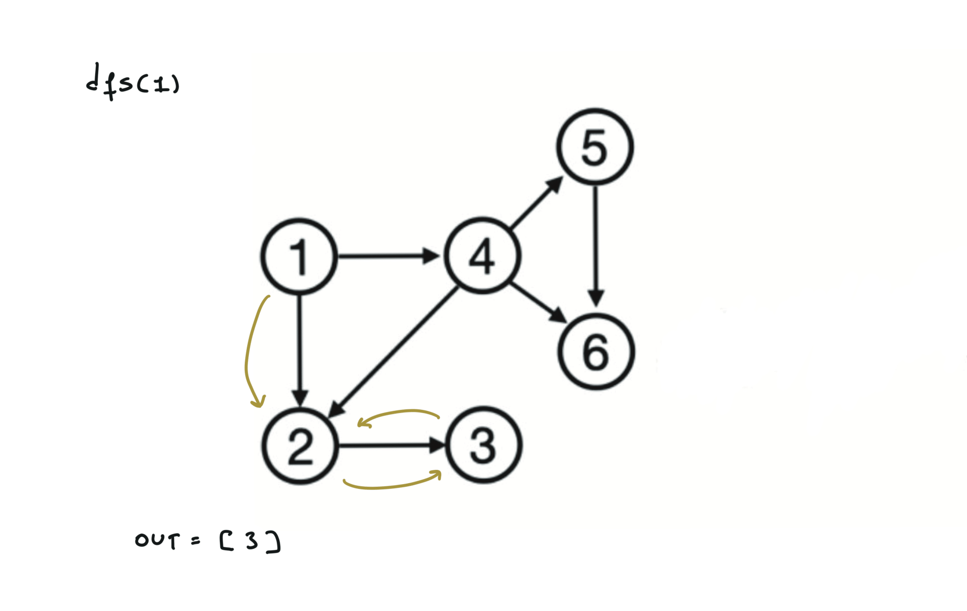
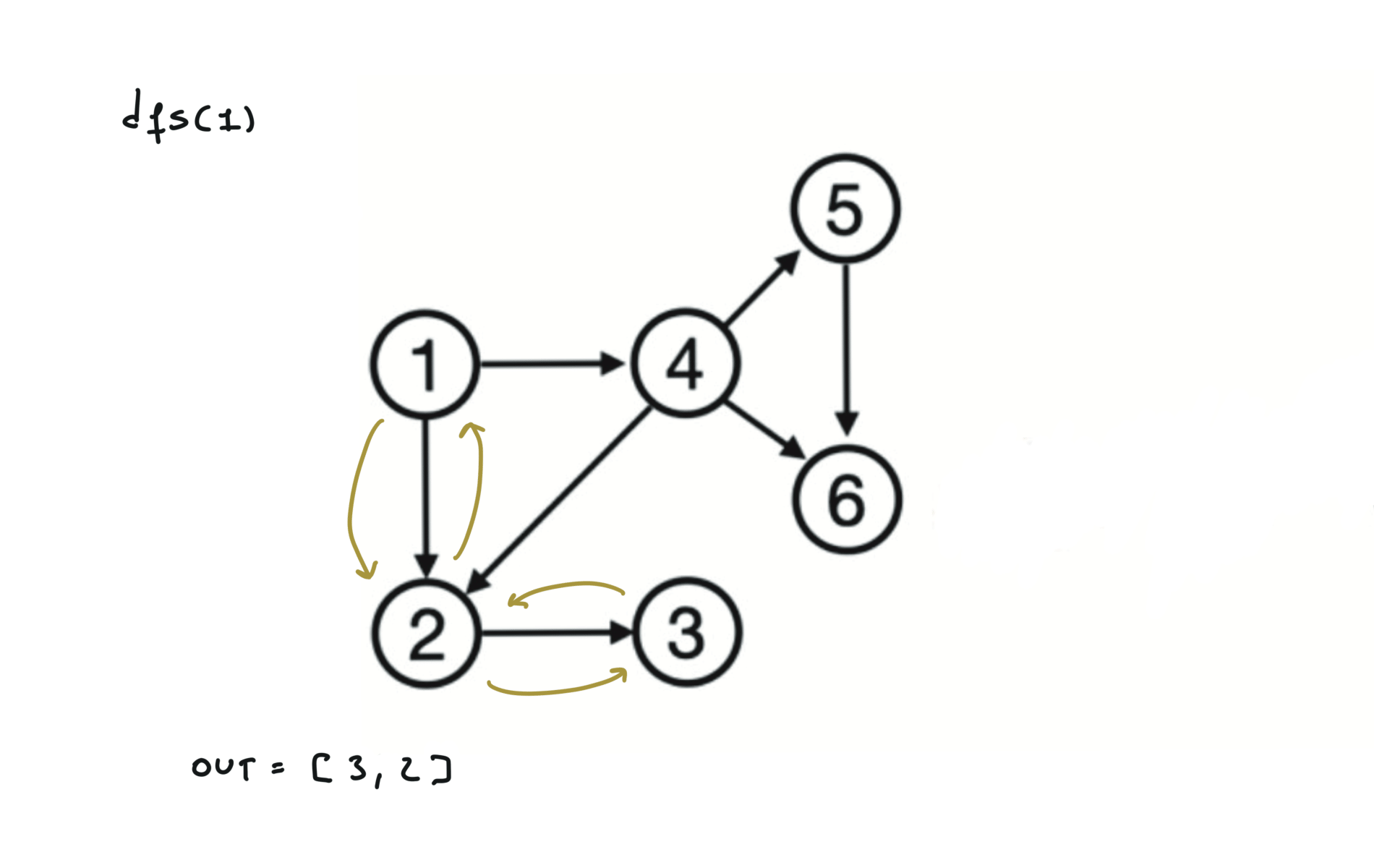
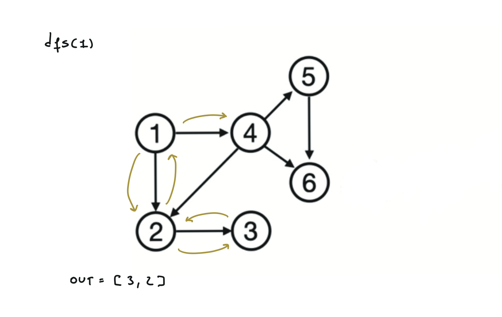
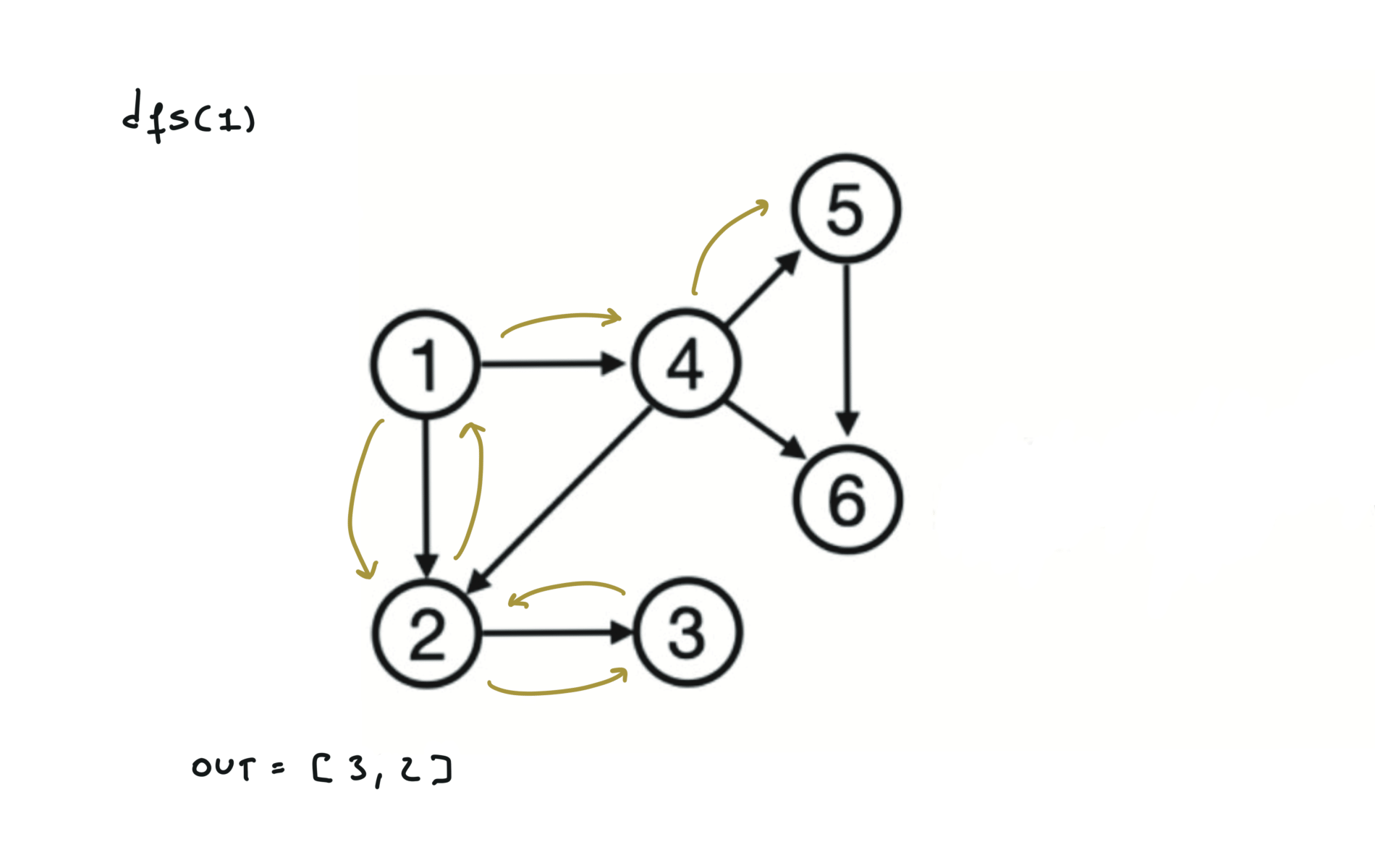
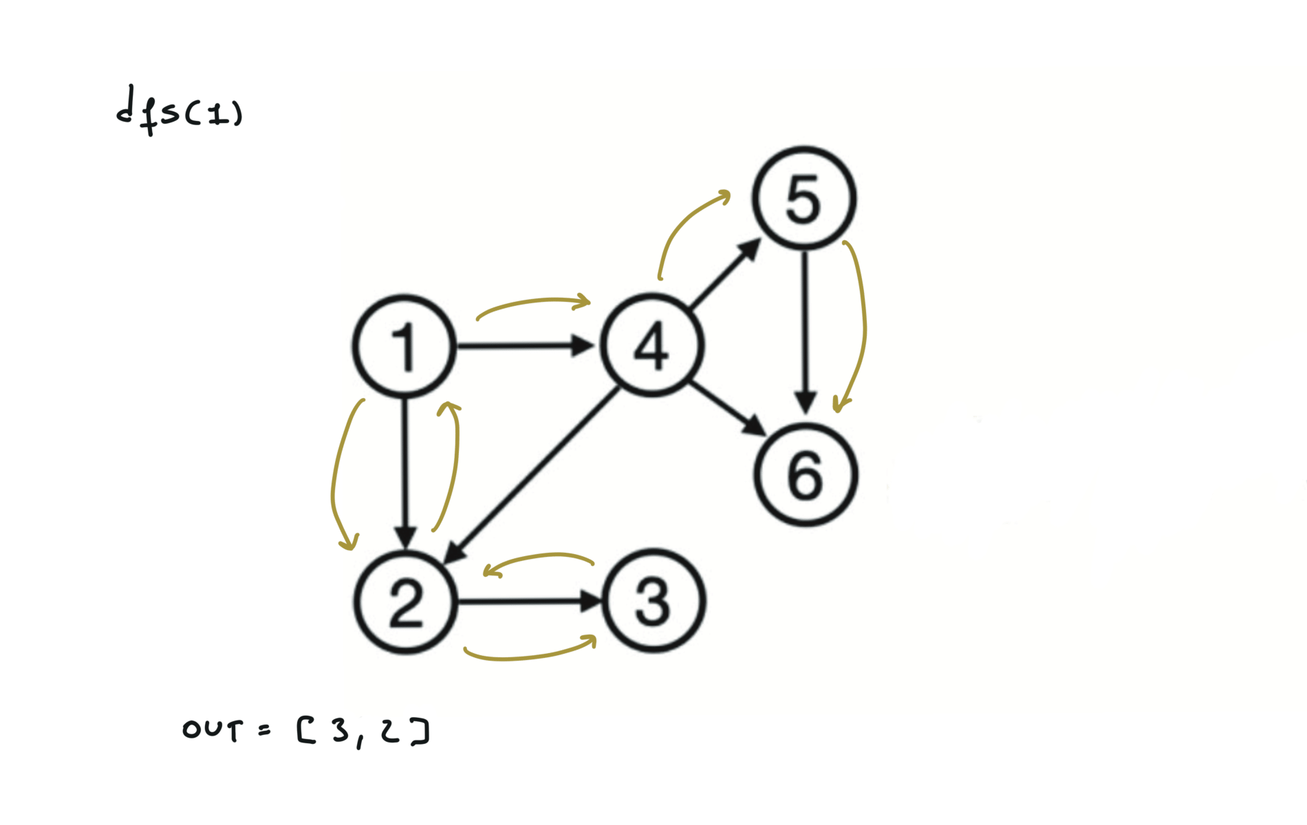
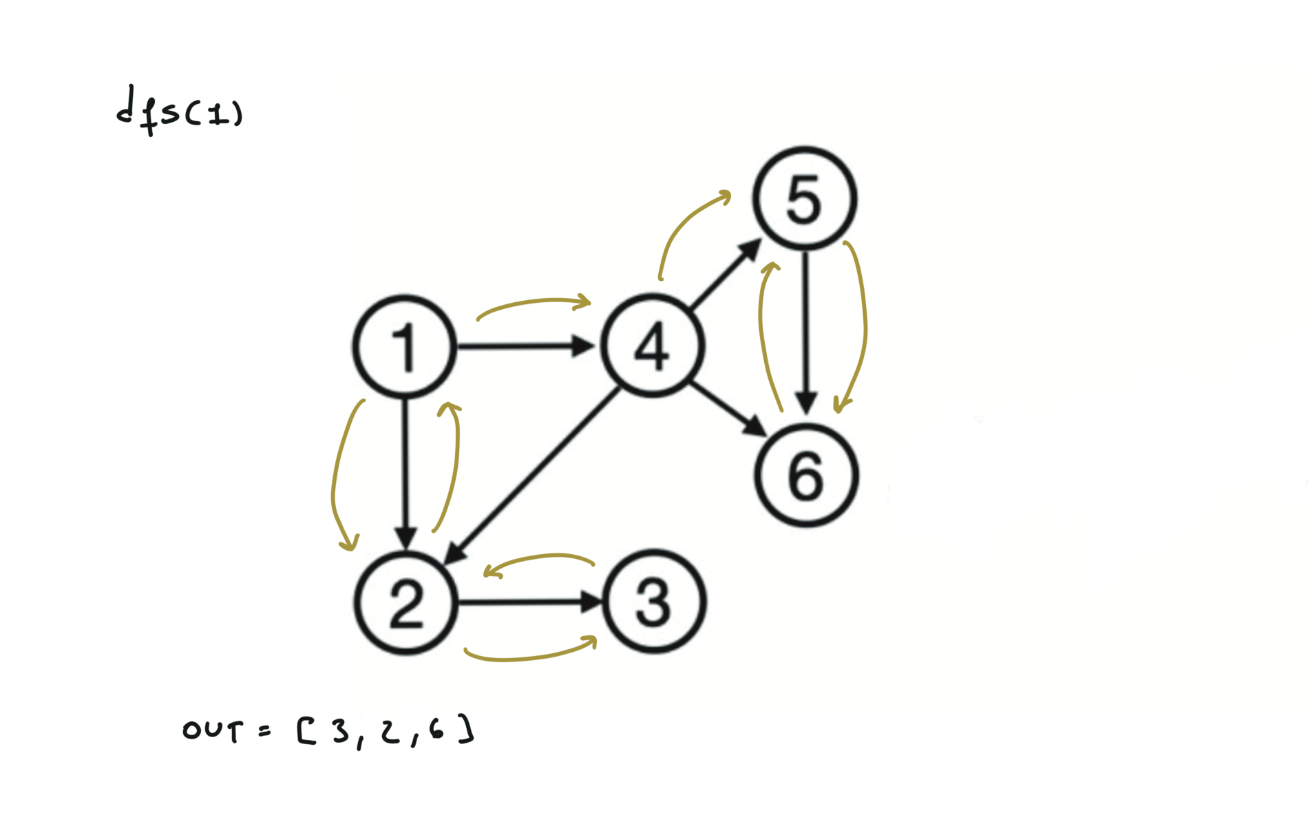
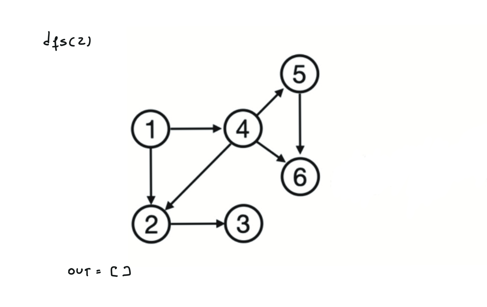
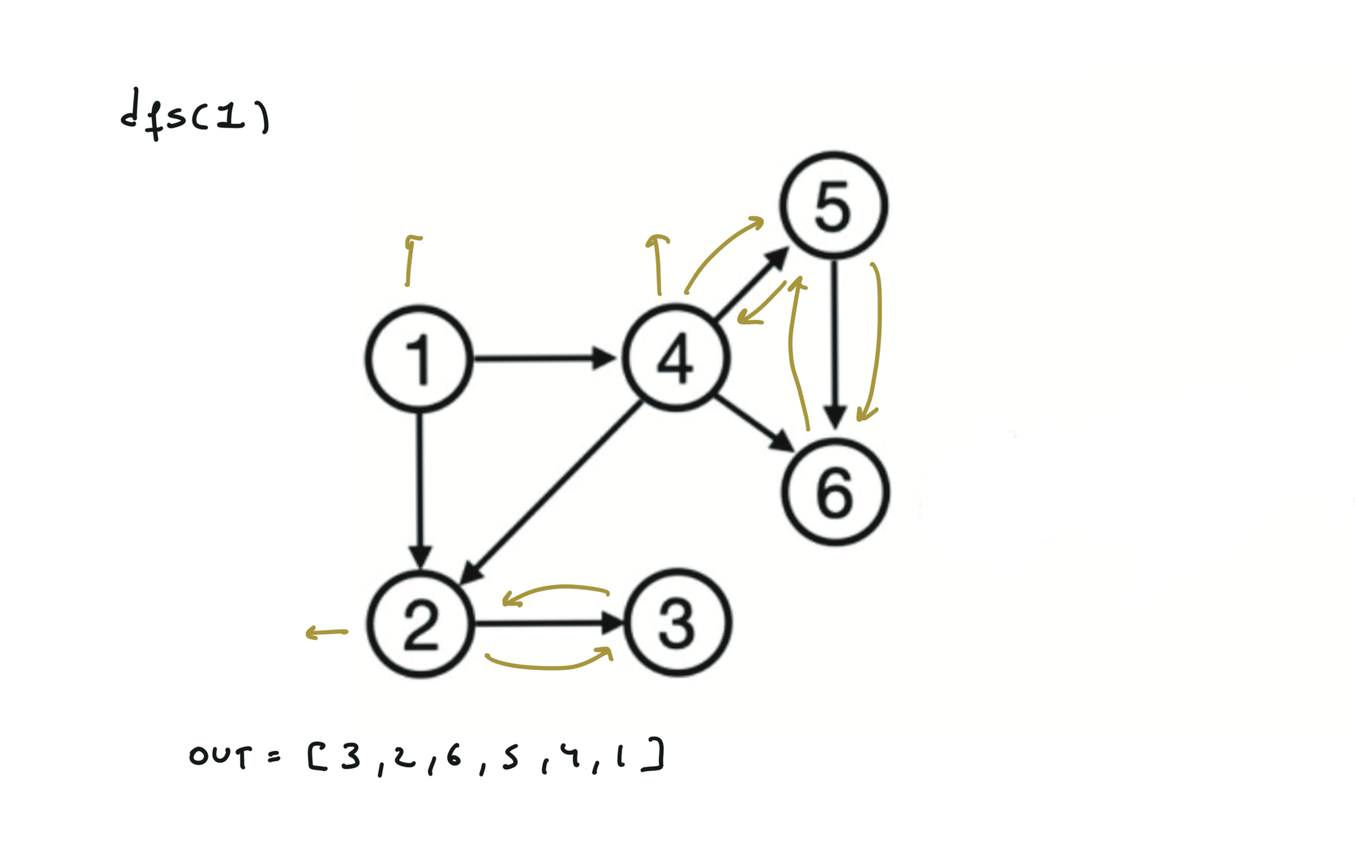
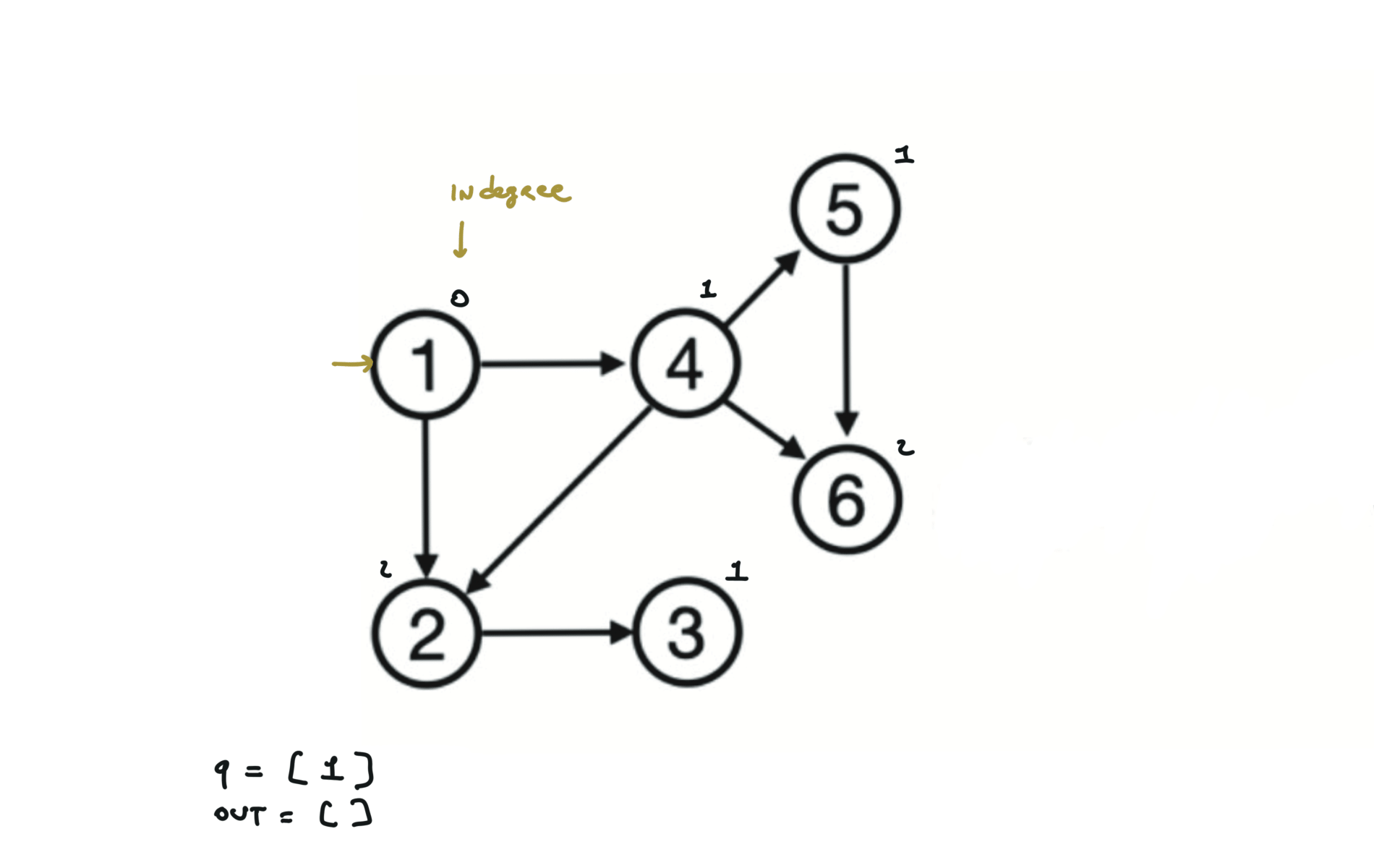
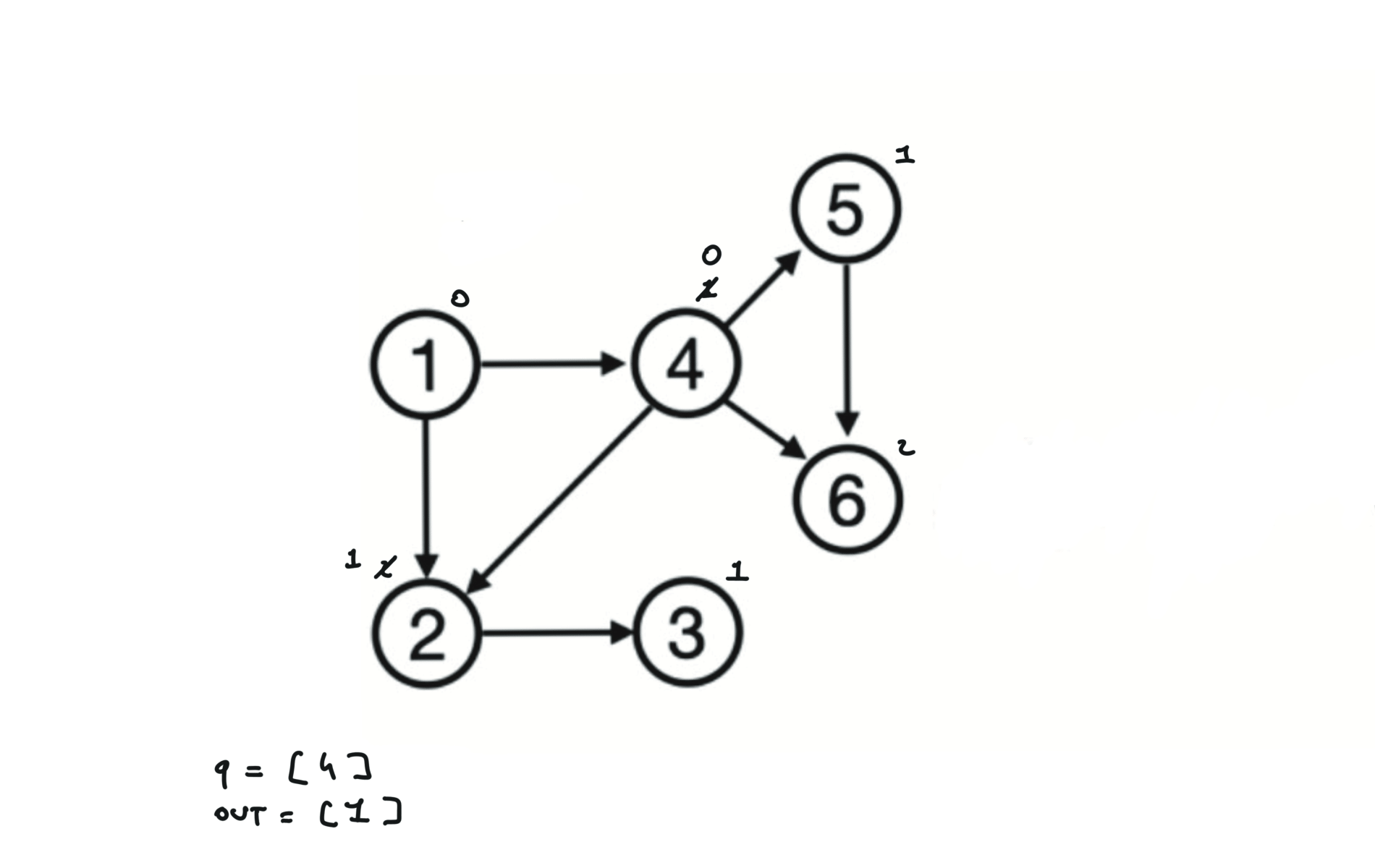
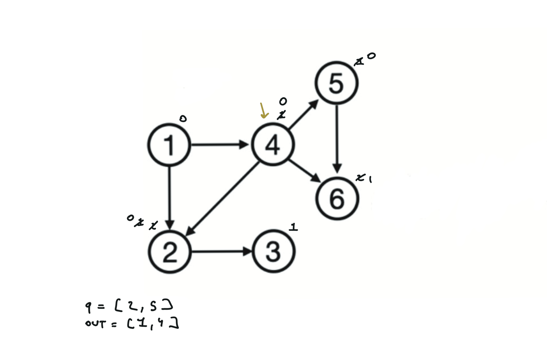
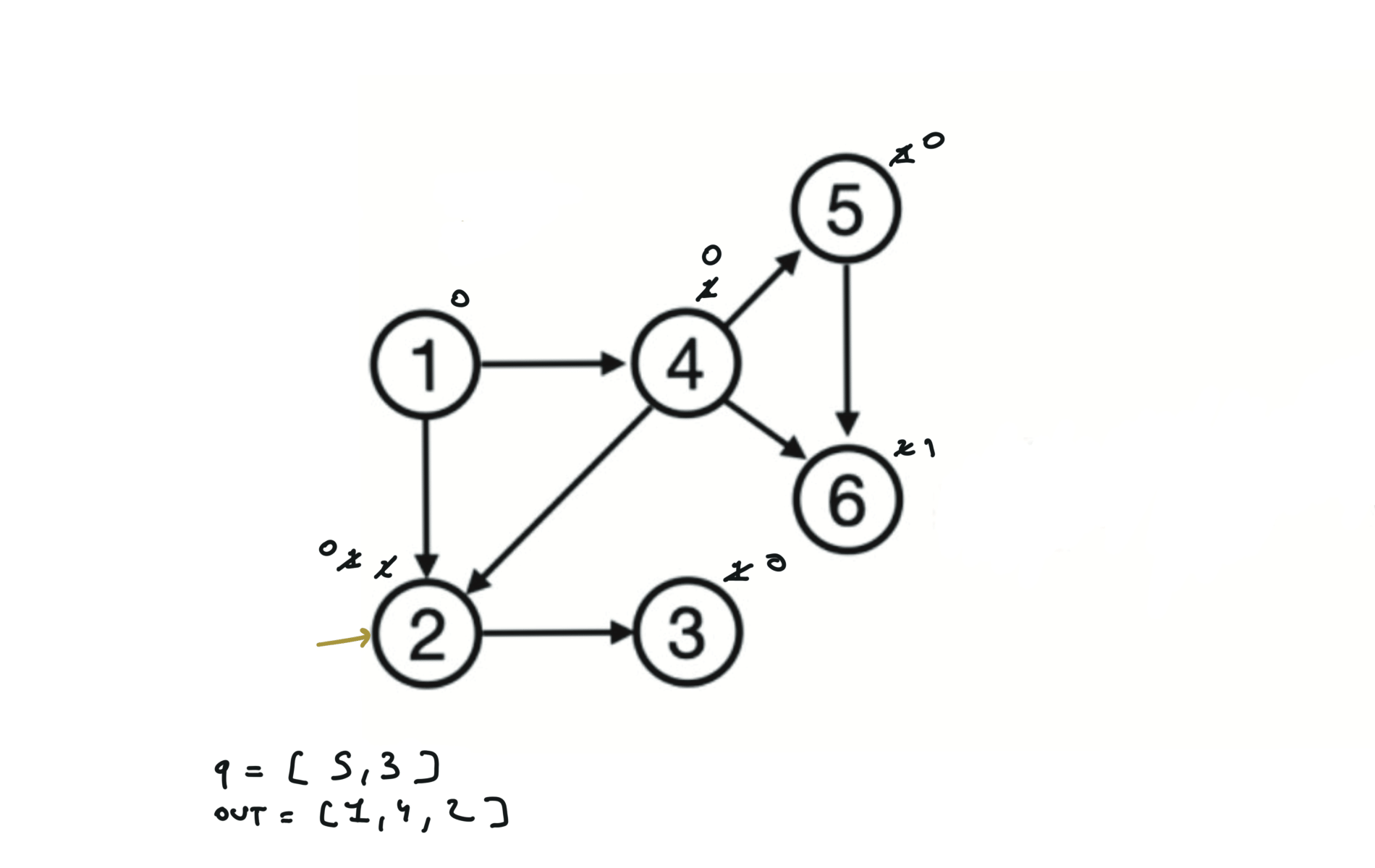
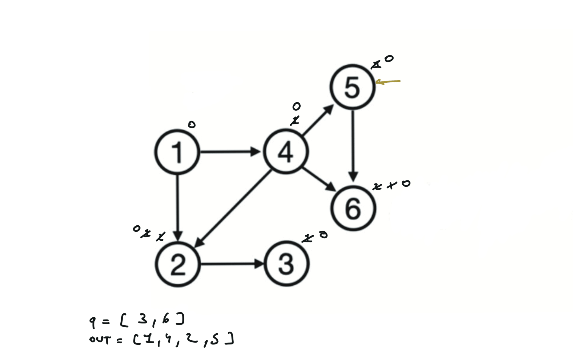
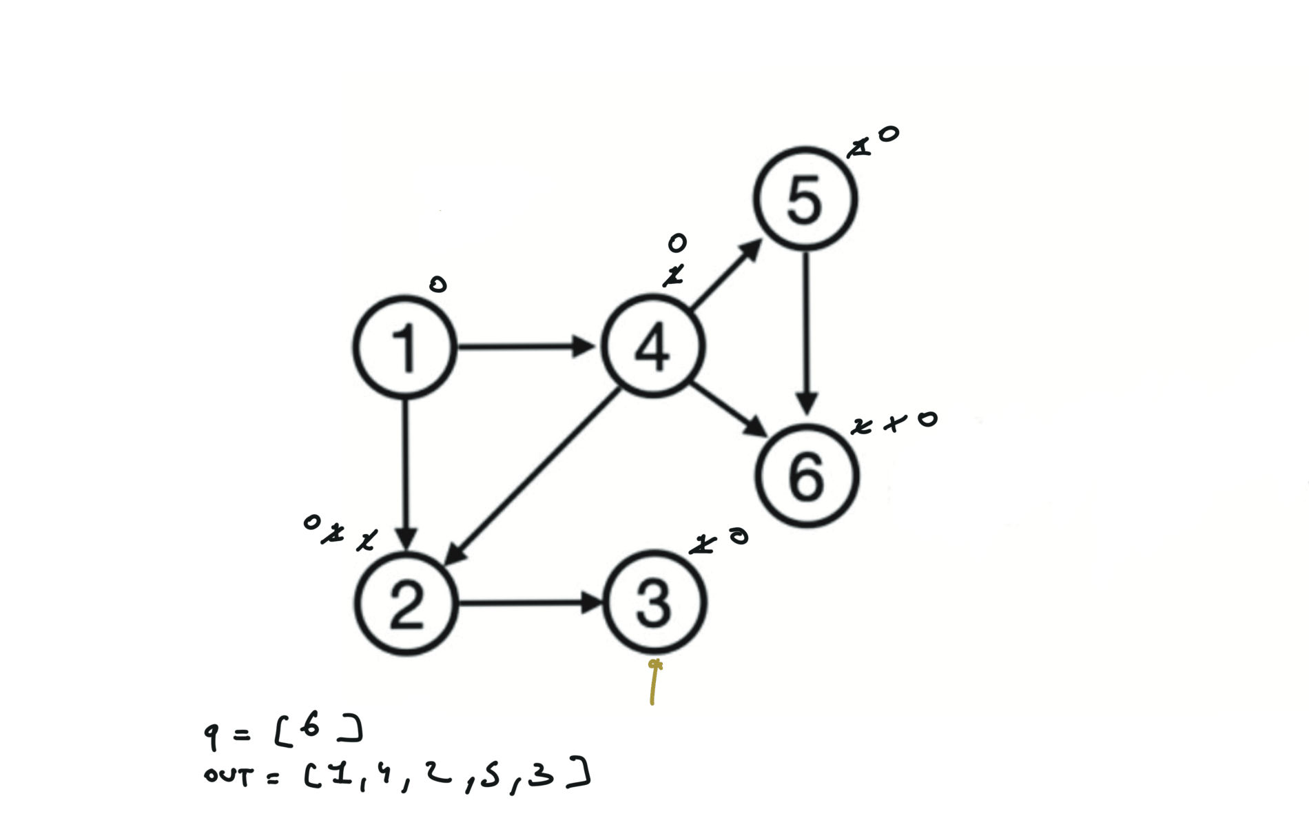
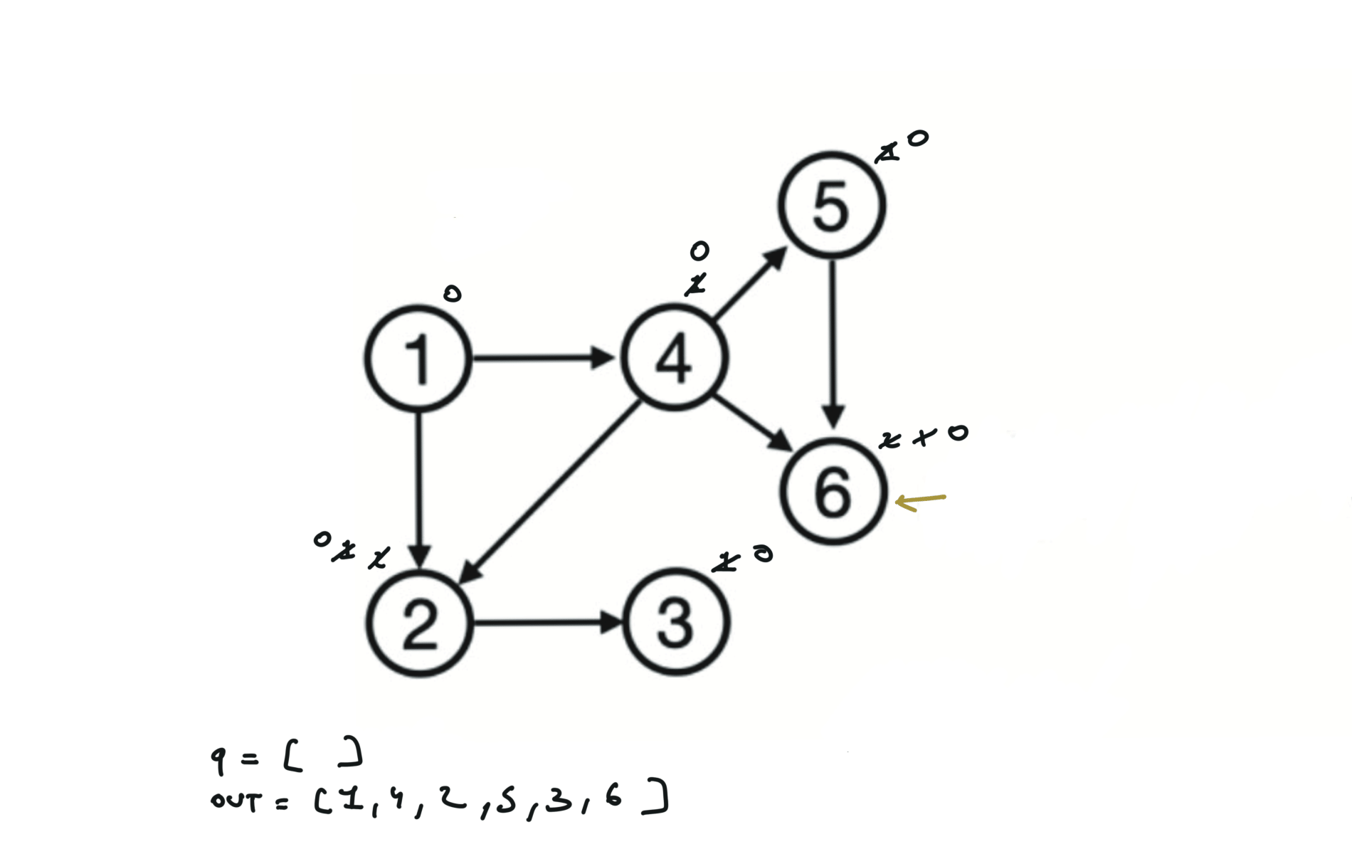
Given a DAG (directed acyclic graph) a topological sort is a linear ordering of all vertices such that for any edge (u, v), u comes before v in the ordering. So a topological ordering for the graph in the photo is: $[1,4,2,3,5,6]$.
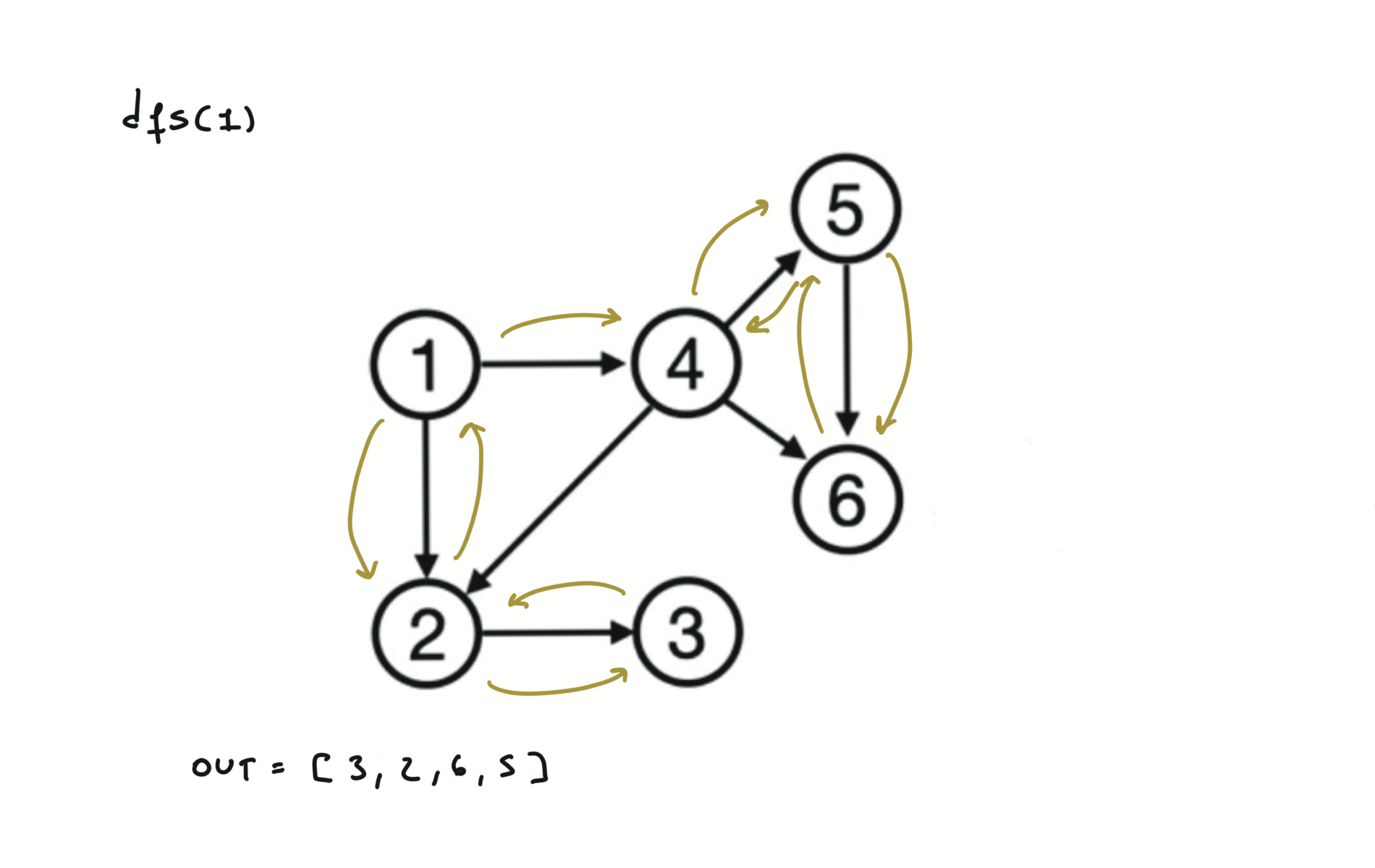
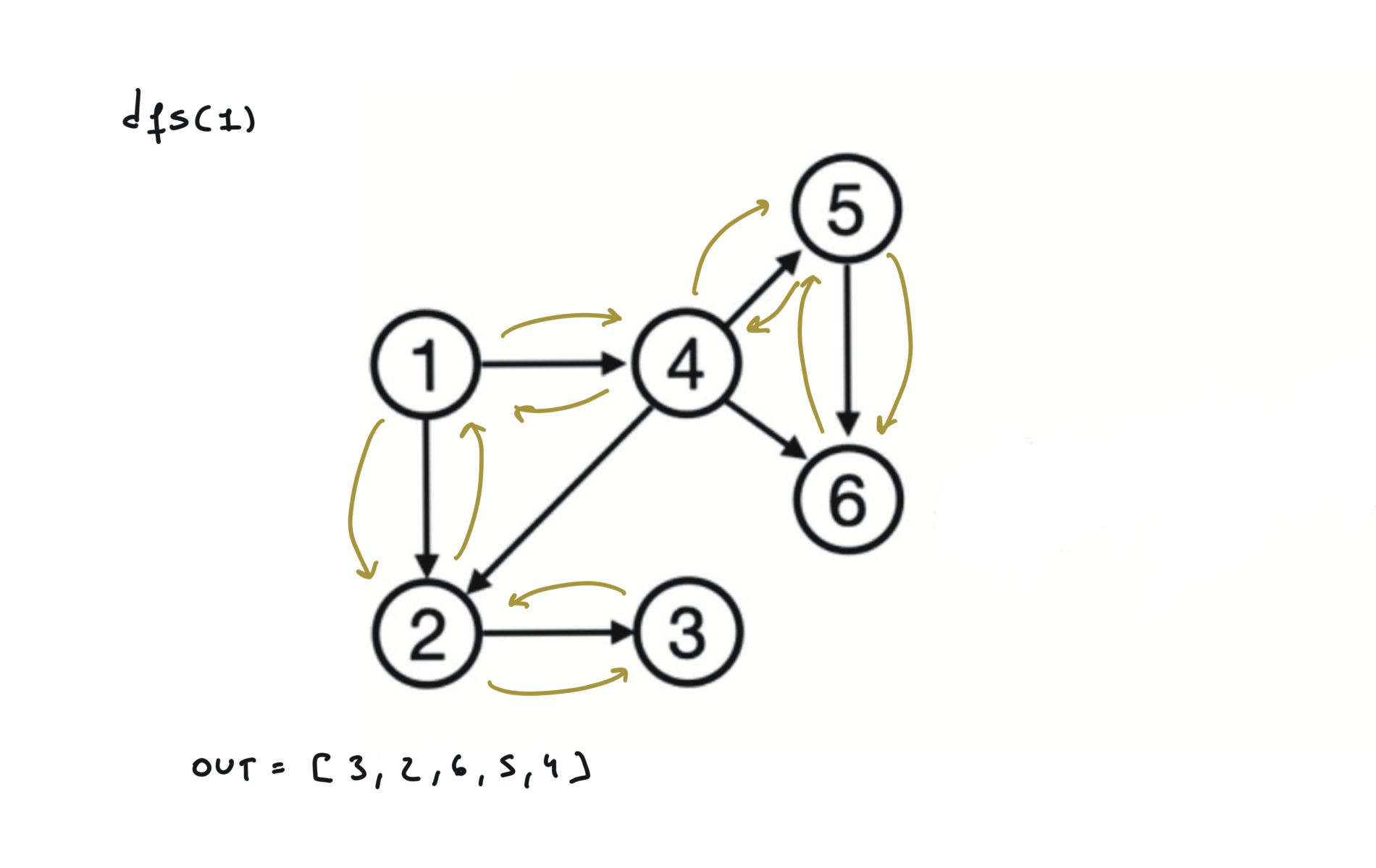
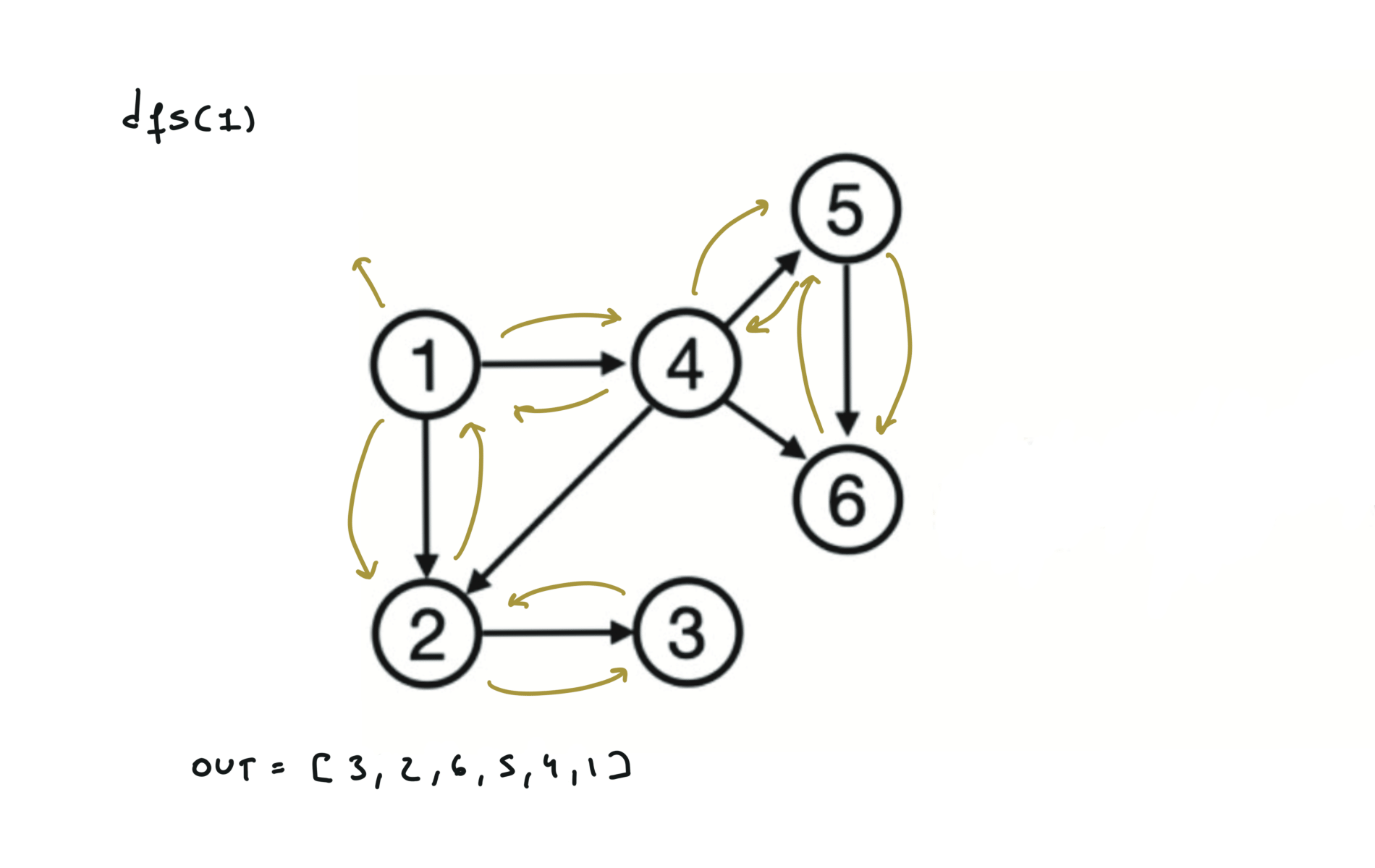
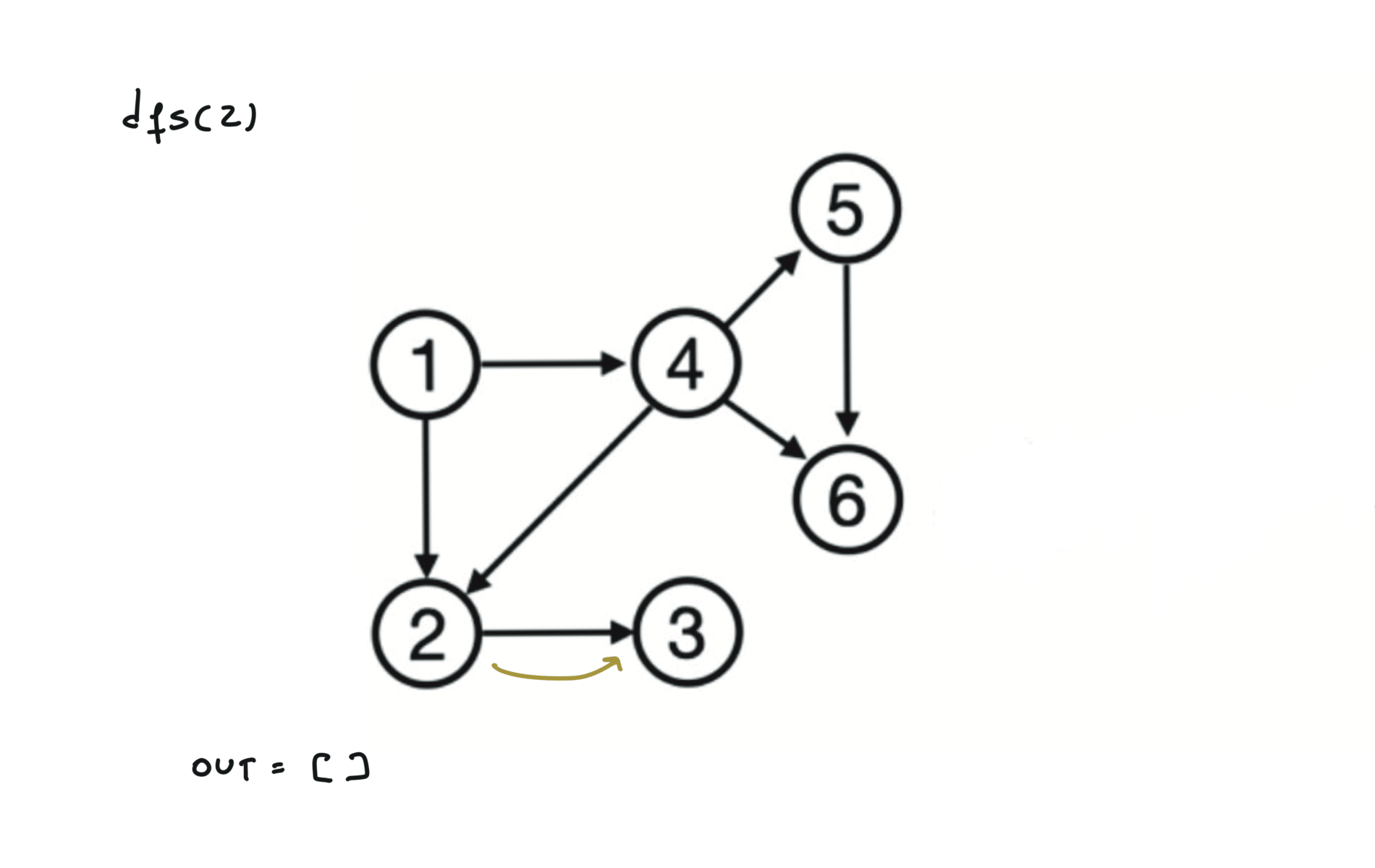
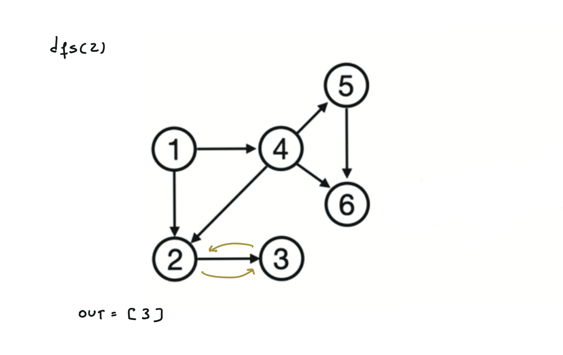
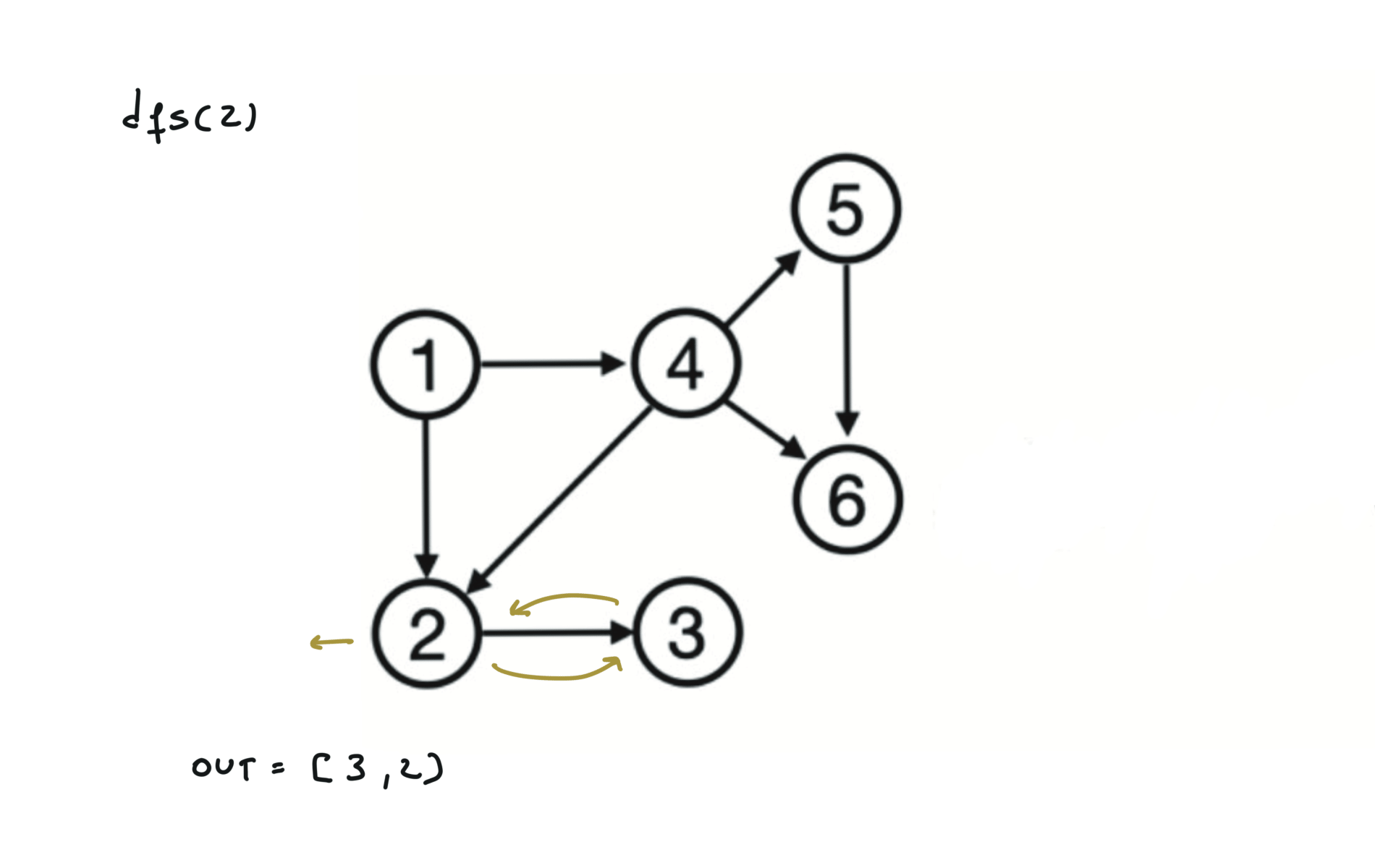
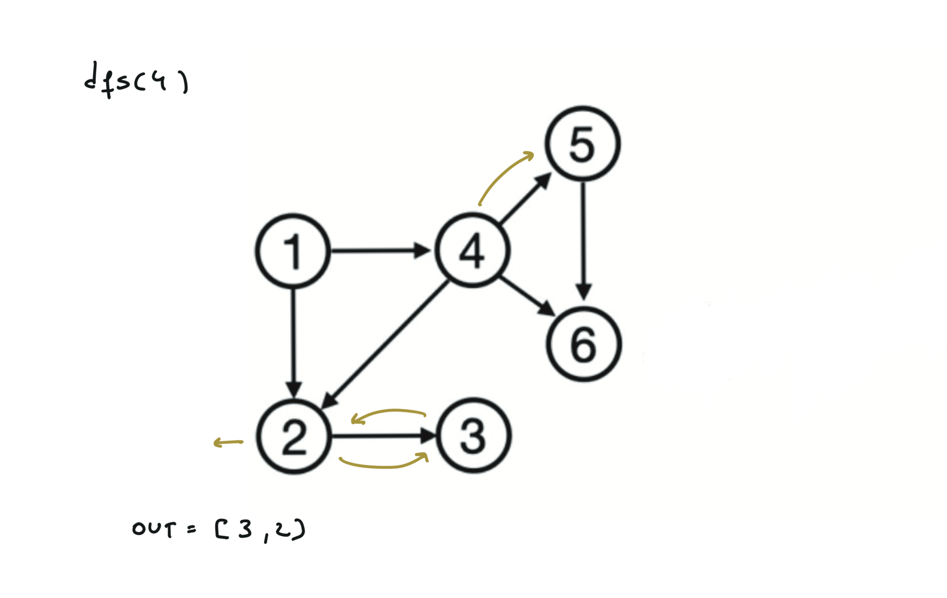
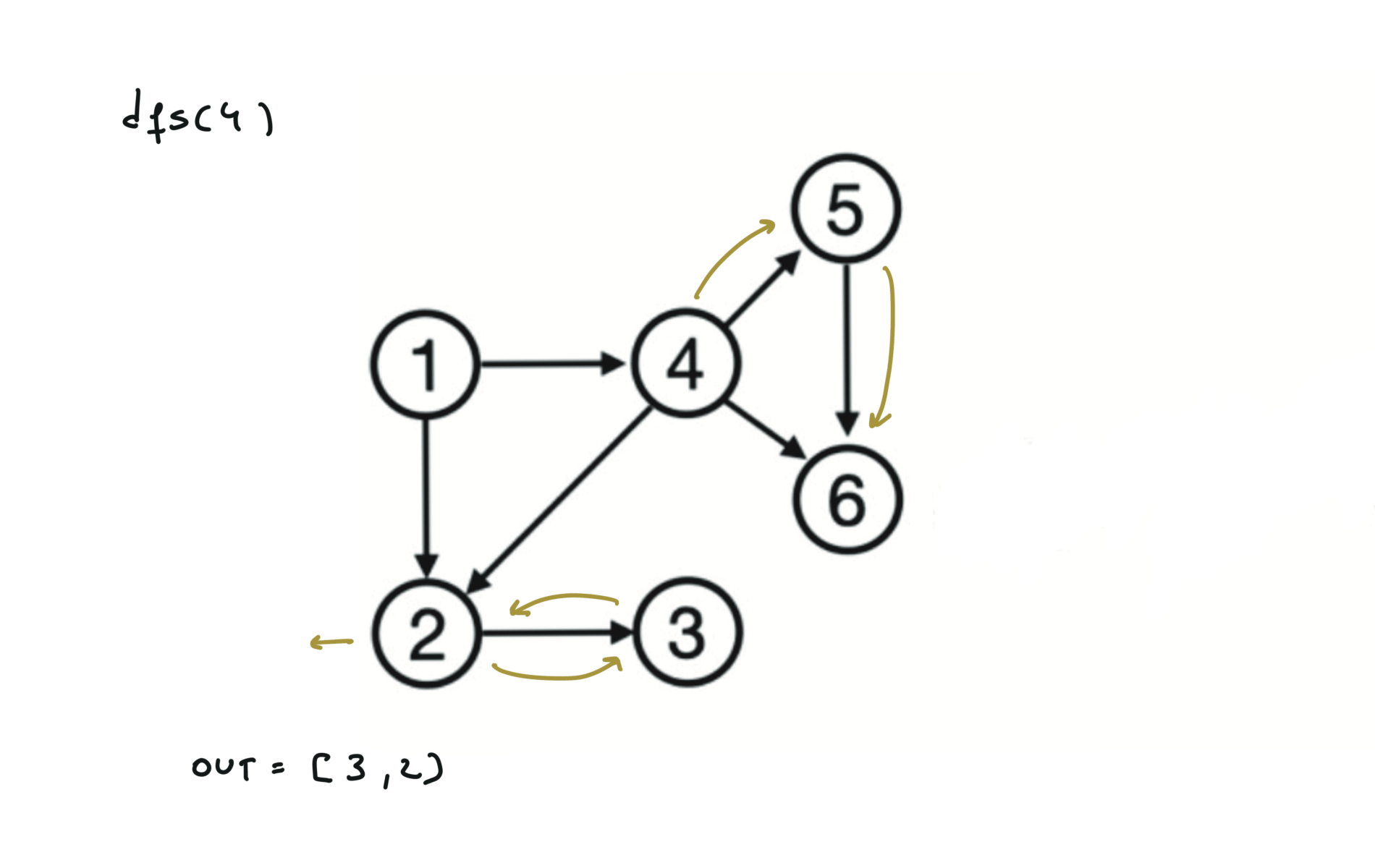
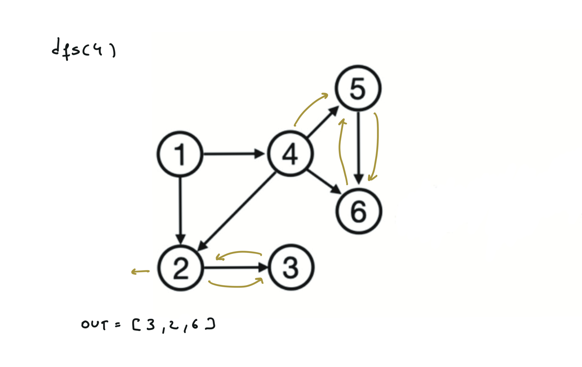
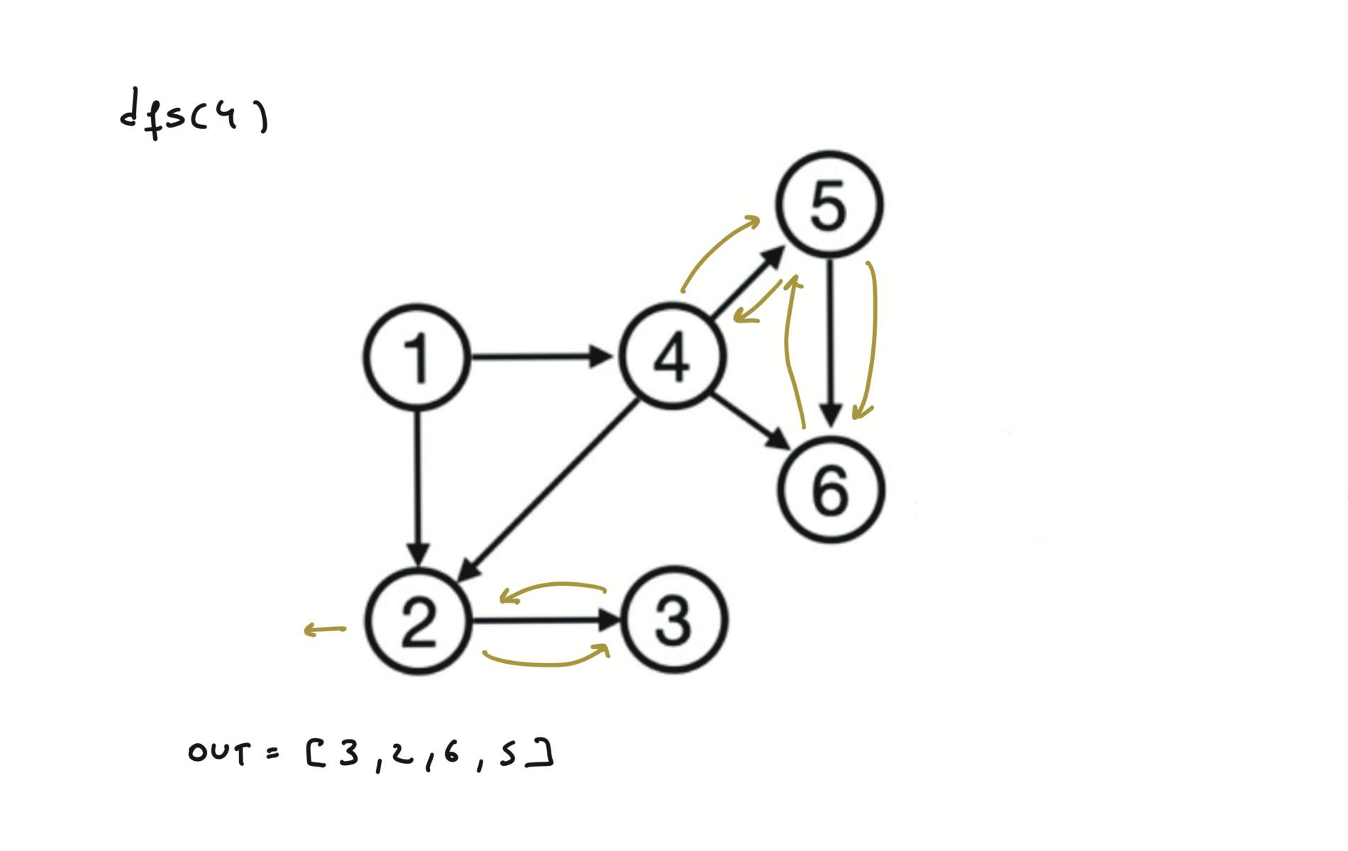
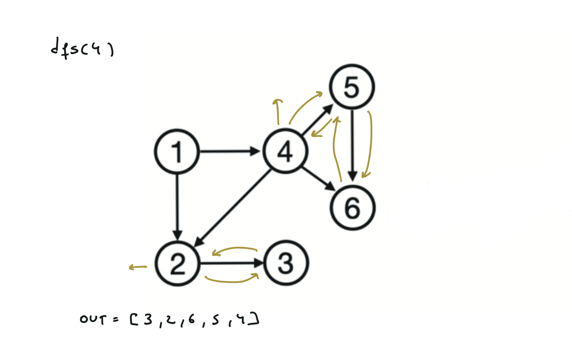
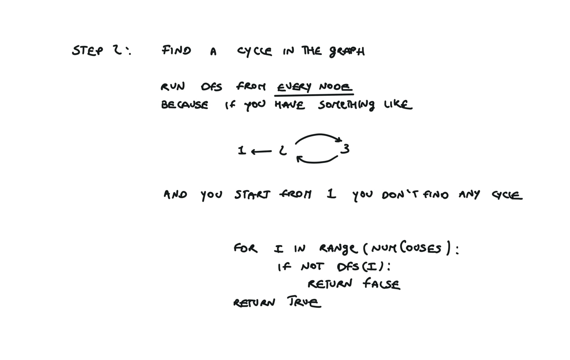
There are other possible topological ordering, for example $[1,4,5,6,2,3]$. Be aware This DFS algorithm runs fine and outputs a order for a graph even if the graph contains cycles. If you want an algorithm that can create a topological ordering but also detecting if the graph contains a cycle you have to use the BFS solution described below. Let’s see an example of how the algorithm works: The outuput does not depend on the node we start with. This is because we loop through all nodes and we run dfs on them.
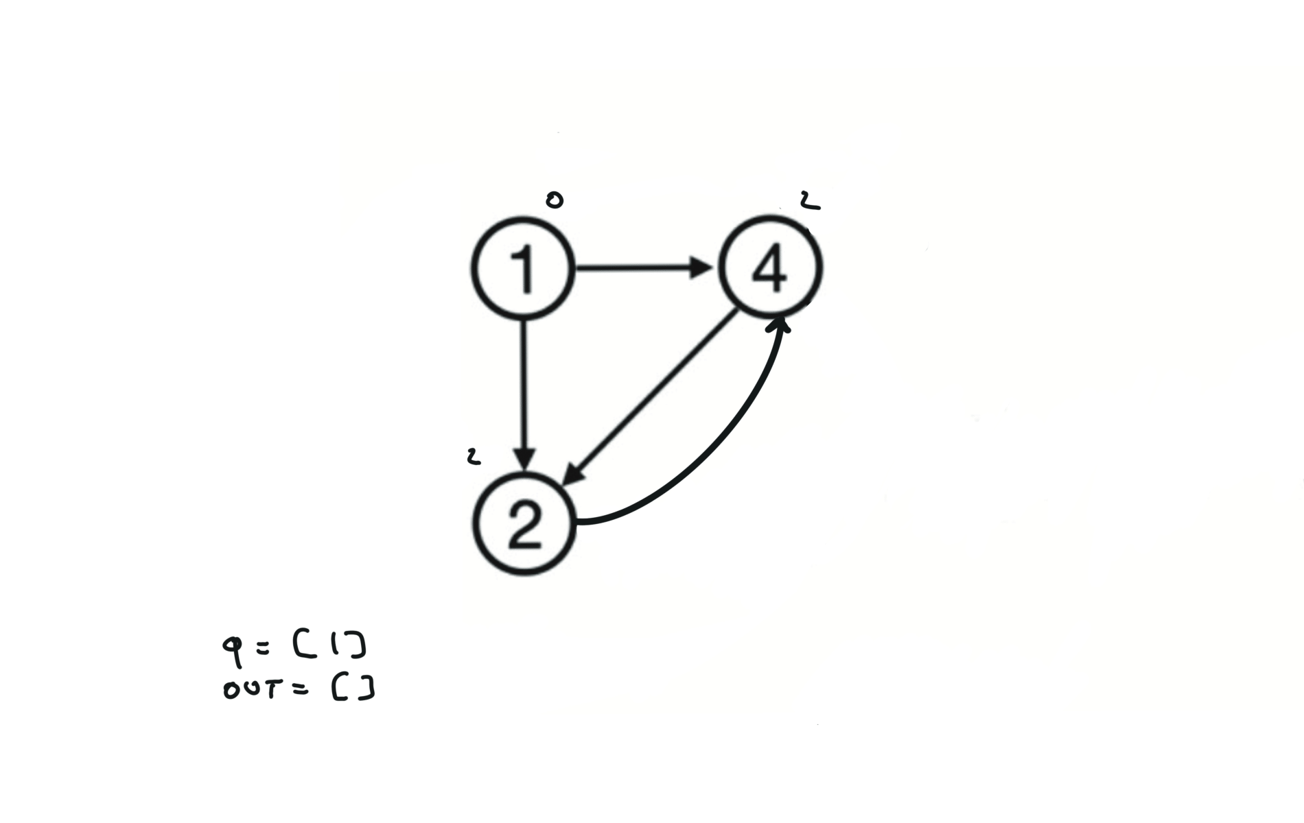
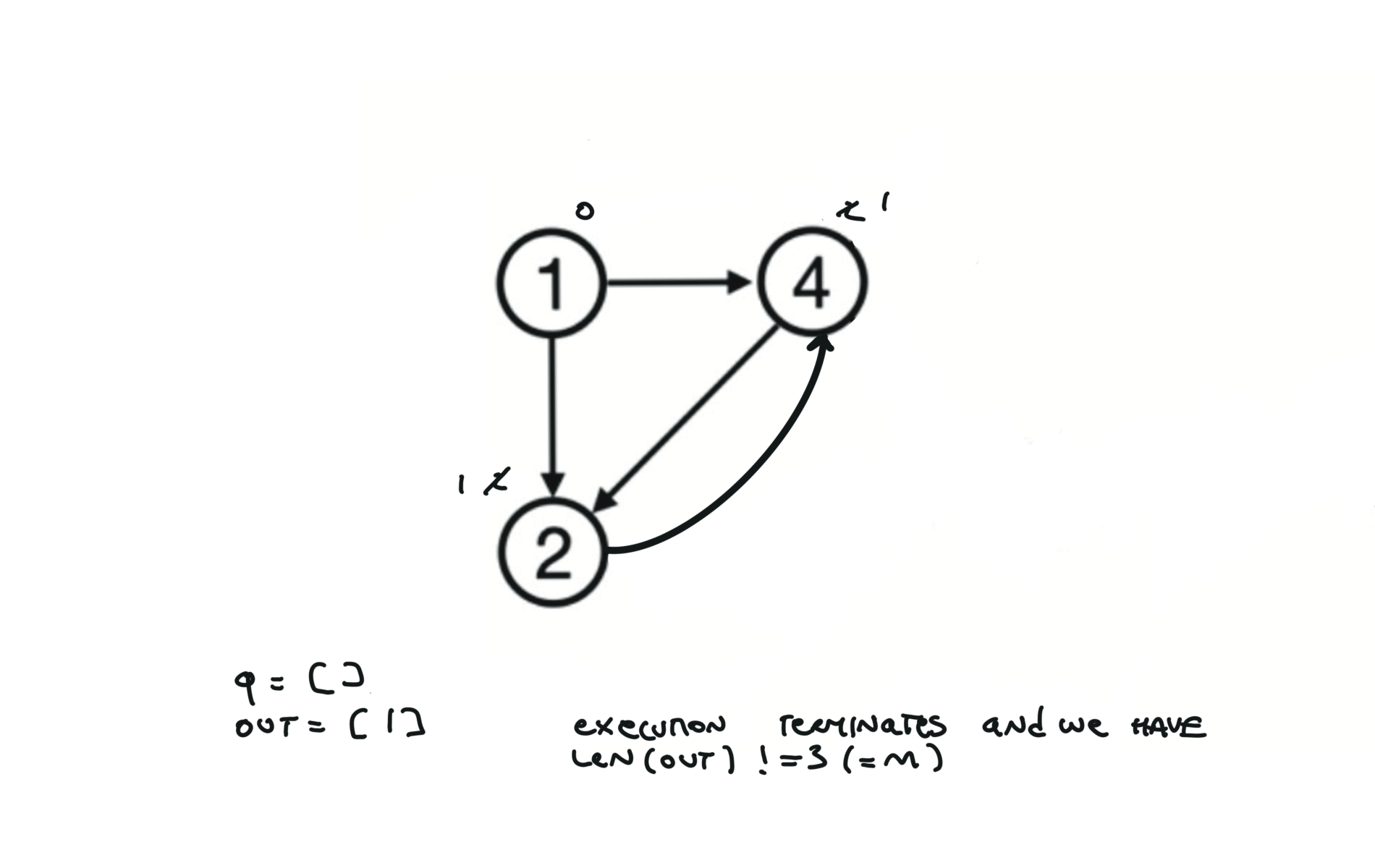
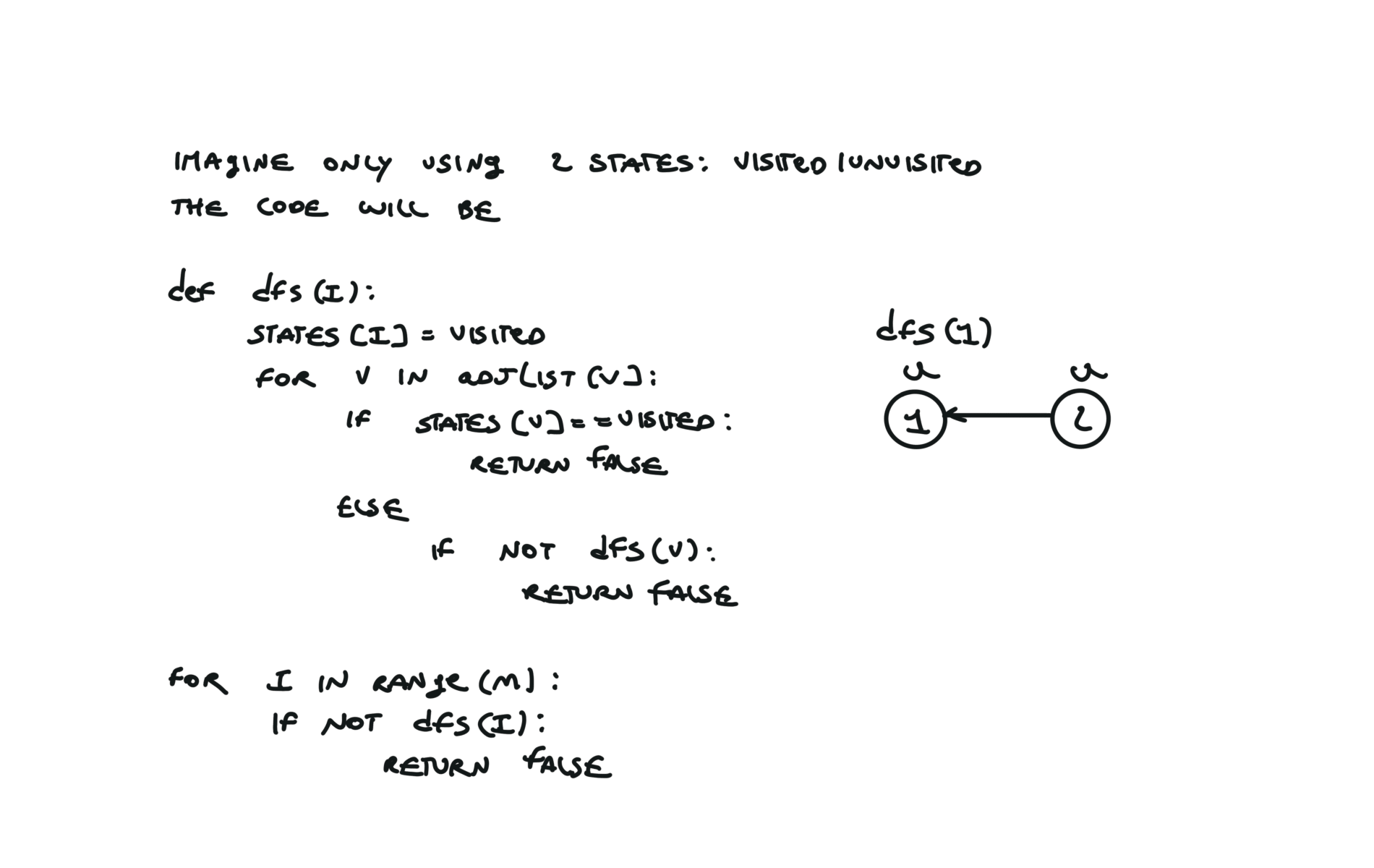
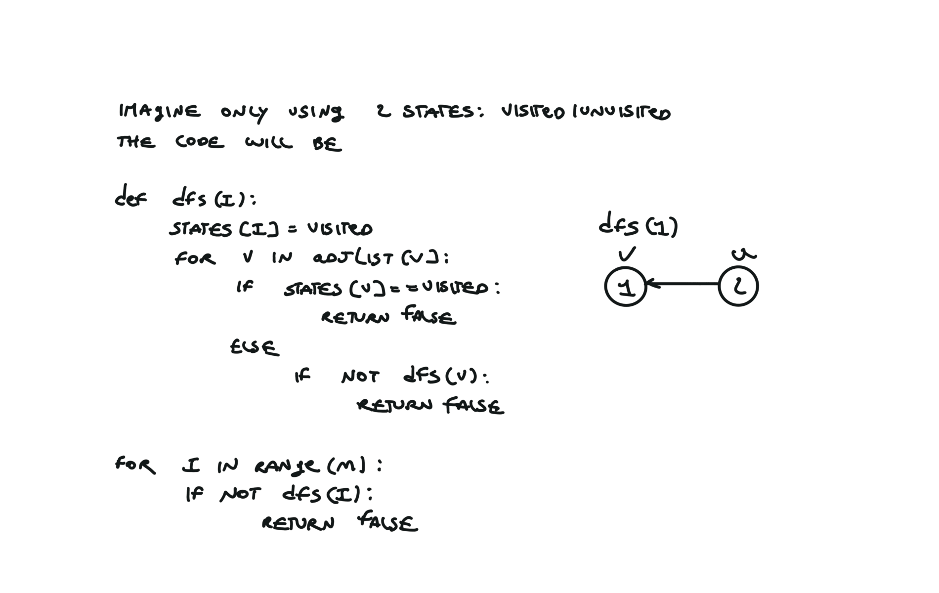
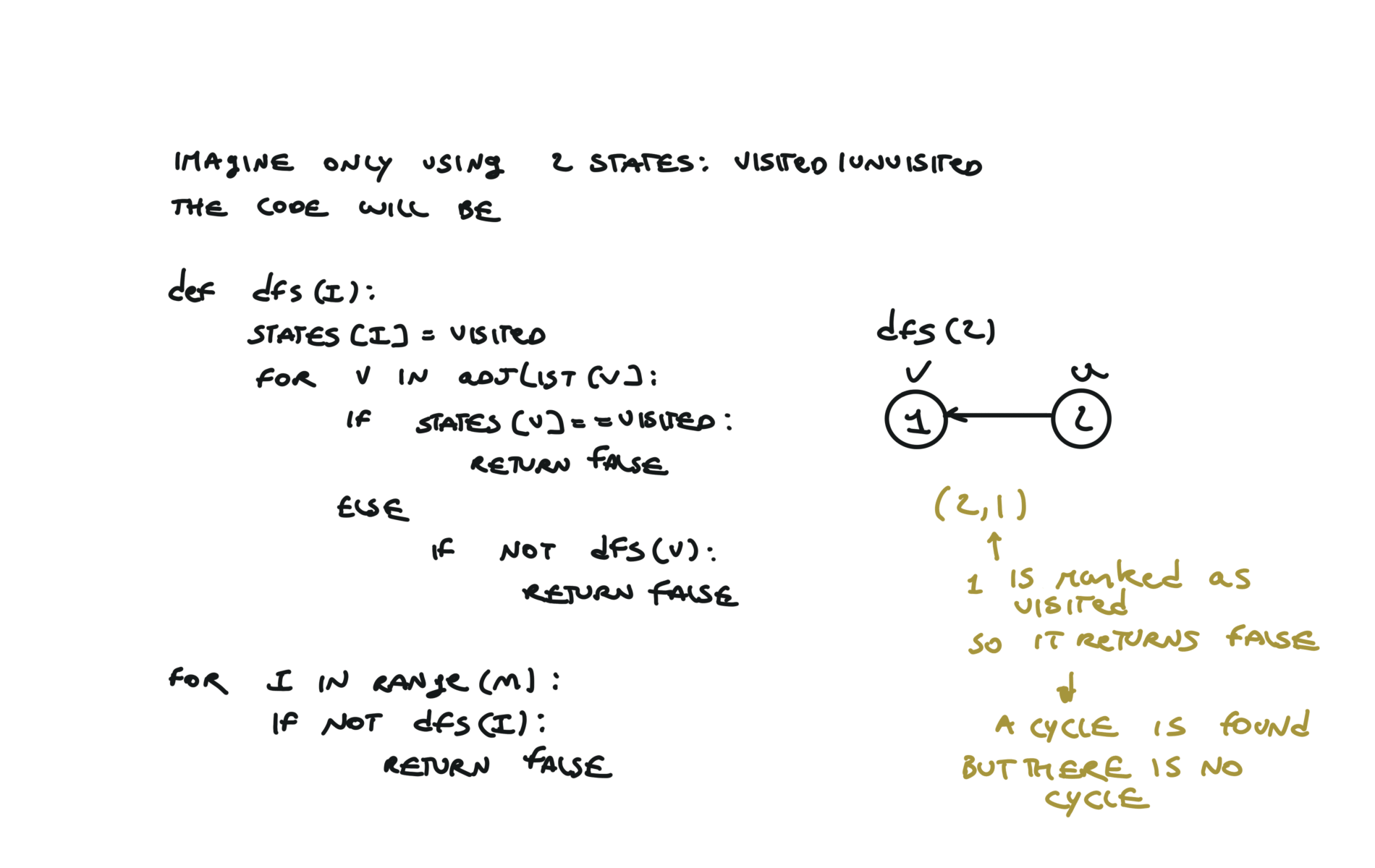
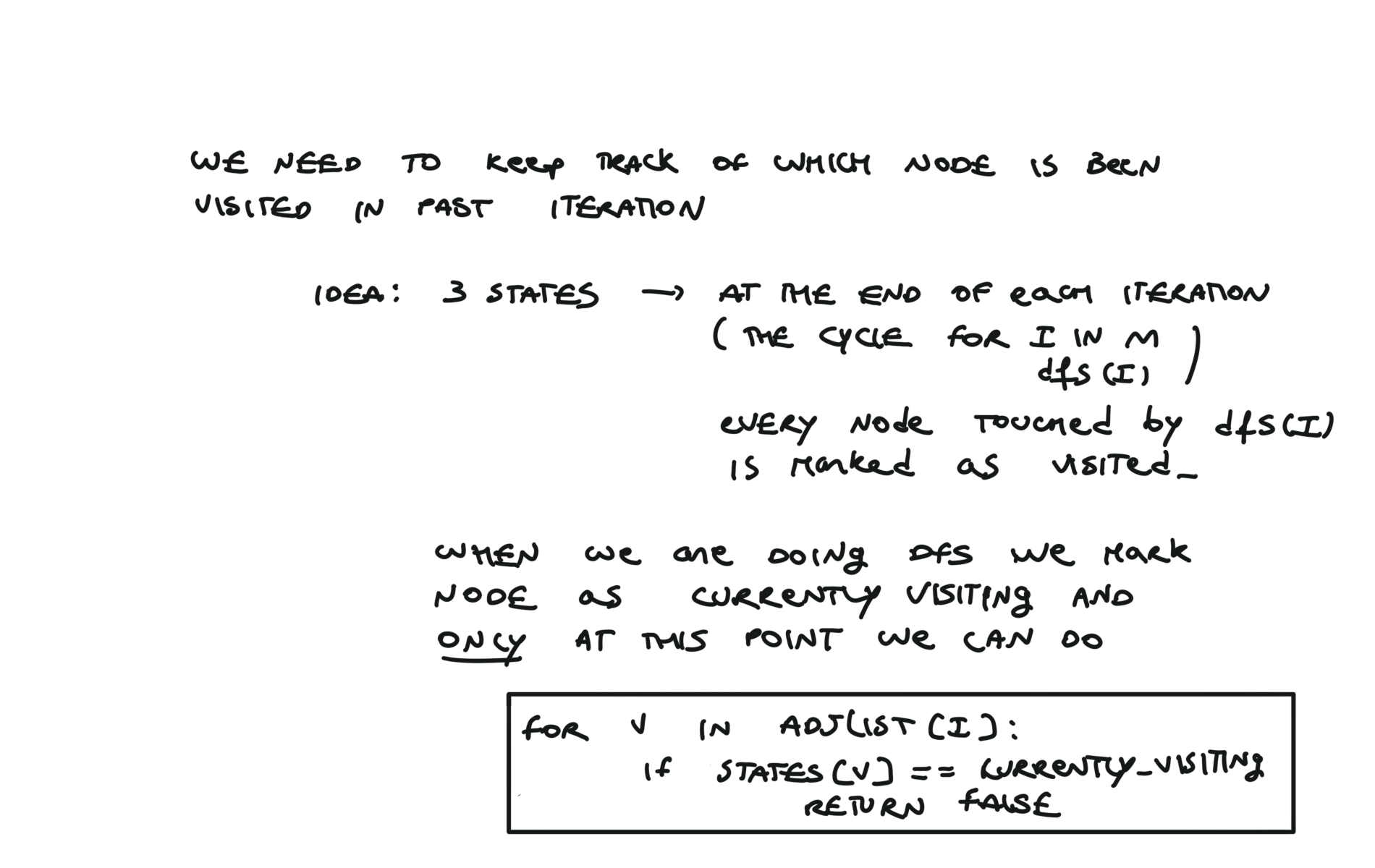
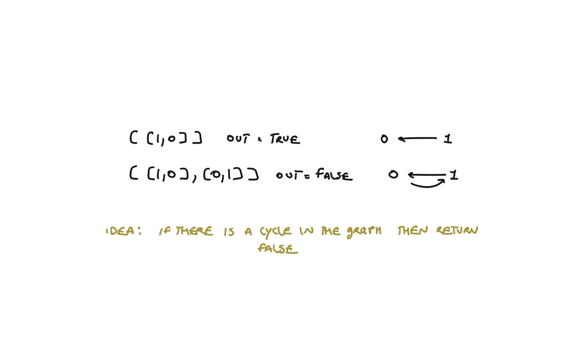
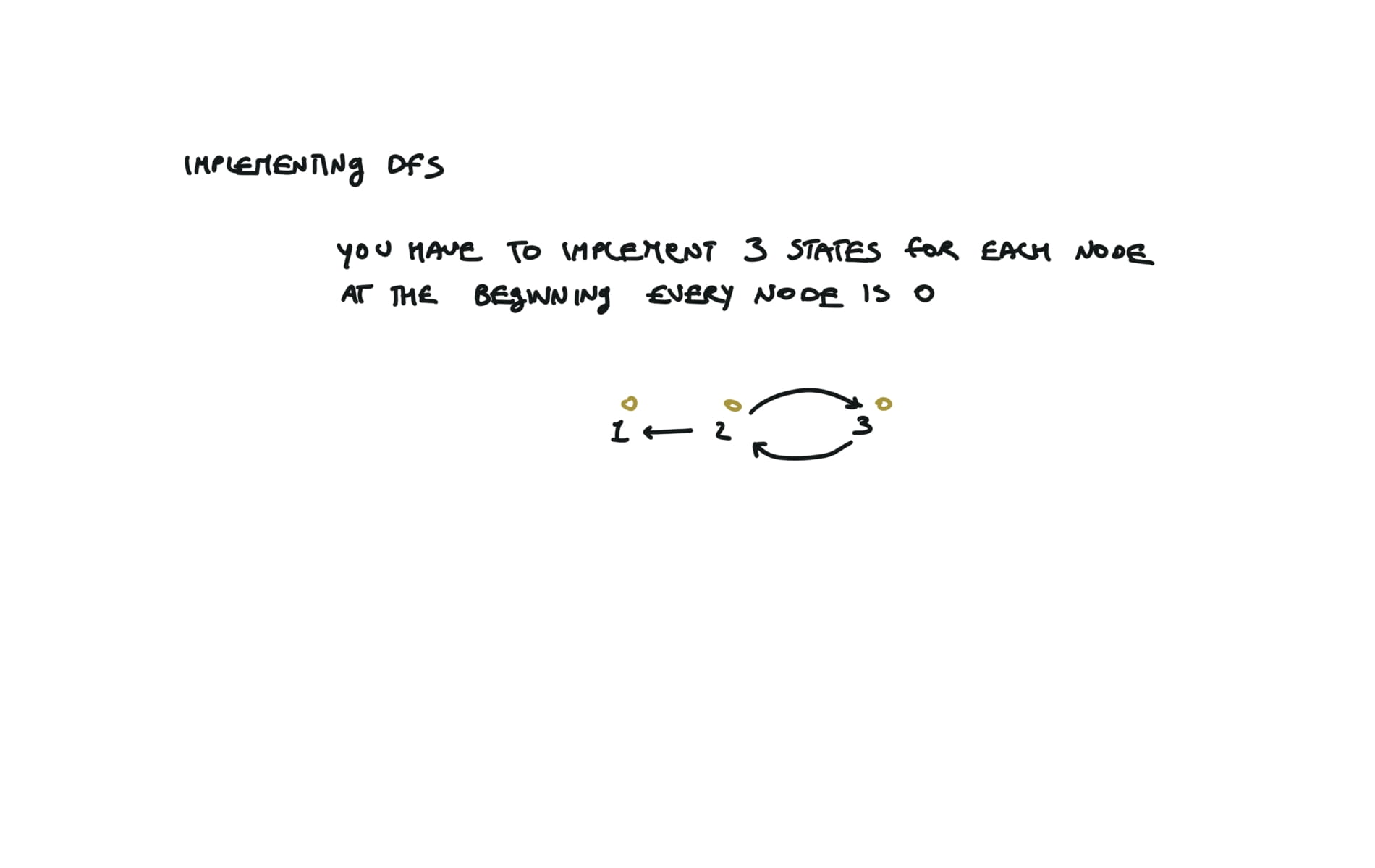
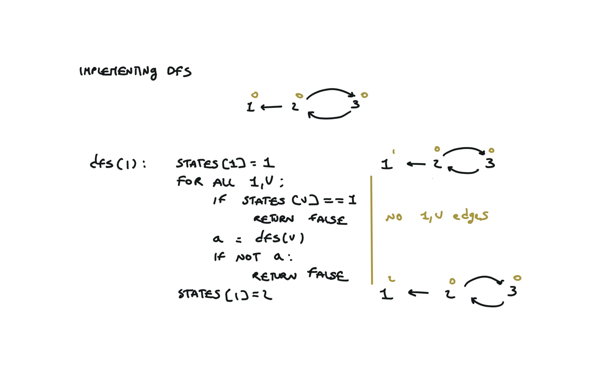
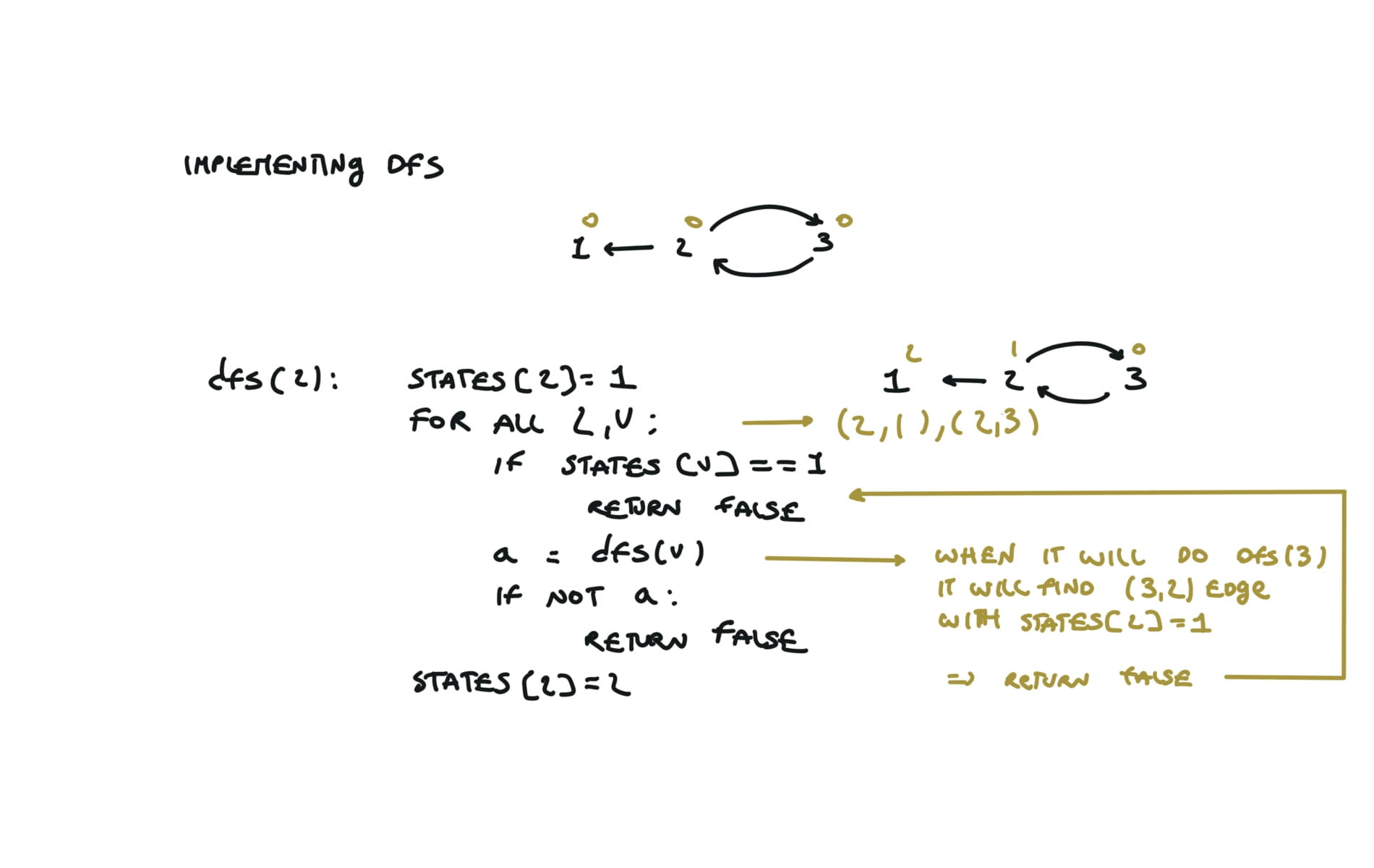
For this reason, let’s see another example, starting from another node. You can see how in the example below: Detecting a cycle in a graph can be implemented using So, instead of only visited/unvisited, we will have 3 states: unvisited/currently being visited/visited.
But why do we need 3 states? Let’s implement the 3 state visit in python:topological sort
using DFS
def dfs(node):
	mark node as visited
	for (node,v) in edges:
		if v not visited:
			dfs(v)
	out.append(node)

out = []
for each node:
	if node not visited:
		dfs(node)
return out.reverse()
using BFS
can be used to detect cycles
indegree = an array indicating indegrees for each node
queue = []
# Add to the BFS queue all nodes with indegree 0
for i in indegree:
    if indegree[i] == 0:
        queue.append(i)

out = []
while q:
	u = q.popleft()
	out.append(u)
	for (u,v) in edges:
		indegree[v] -= 1
		if indegree[v] == 0:
			queue.append(v)

if len(out) == n:
	return out
else:
	return "graphs contains a cycle"
Topological ordering with BFS can be used to detect cycles
detect cycles
UNVISITED = 0
CURRENTLY_VISITING = 1
VISITED = 2
states = [0] * numCourses
def dfs(i):
    if states[i] == VISITED:
        return True
    states[i] = CURRENTLY_VISITING
    for v in adjList[i]:
        if states[v] == CURRENTLY_VISITING:
            return False
        a = dfs(v)
         if not a:
            return False
    states[i] = VISITED
    return True

for i in range(numCourses):
    if not dfs(i):
        return False
return True
200. Number of Islands
[desc]
(link)
def bfs(i,j):
    q = deque([(i,j)])
    grid[i][j] = '0'
    while q:
        r,c = q.popleft()
        if r+1 in range(len(grid)) and grid[r+1][c] == '1':
            q.append((r+1,c))
            grid[r+1][c] = '0'
        if r-1 in range(len(grid)) and grid[r-1][c] == '1':
            q.append((r-1,c))
            grid[r-1][c] = '0'
        if c+1 in range(len(grid[0])) and grid[r][c+1] == '1':
            q.append((r,c+1))
            grid[r][c+1] = '0'
        if c-1 in range(len(grid[0])) and grid[r][c-1] == '1':
            q.append((r,c-1))
            grid[r][c-1] = '0'
count = 0
for i in range(len(grid)):
	for j in range(len(grid[0])):
        if grid[i][j] == '1':
            bfs(i,j)
            count +=1
return count
DFS solution
def dfs(self, grid, i, j):
	if i<0 or j<0 or i>=len(grid) or j>=len(grid[0]) or grid[i][j] != '1':
        return
    grid[i][j] = '#'
    self.dfs(grid, i+1, j)
    self.dfs(grid, i-1, j)
    self.dfs(grid, i, j+1)
    self.dfs(grid, i, j-1)

count = 0
for i in range(len(grid)):
    for j in range(len(grid[0])):
        if grid[i][j] == '1':
            self.dfs(grid, i, j)
            count += 1
return count
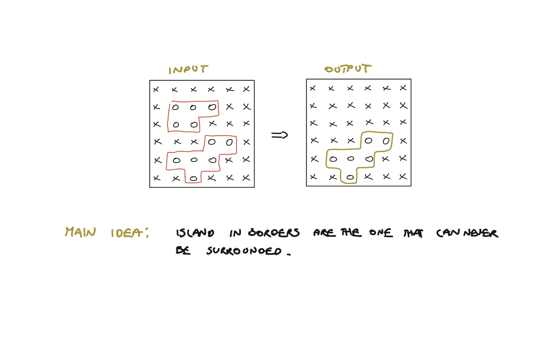
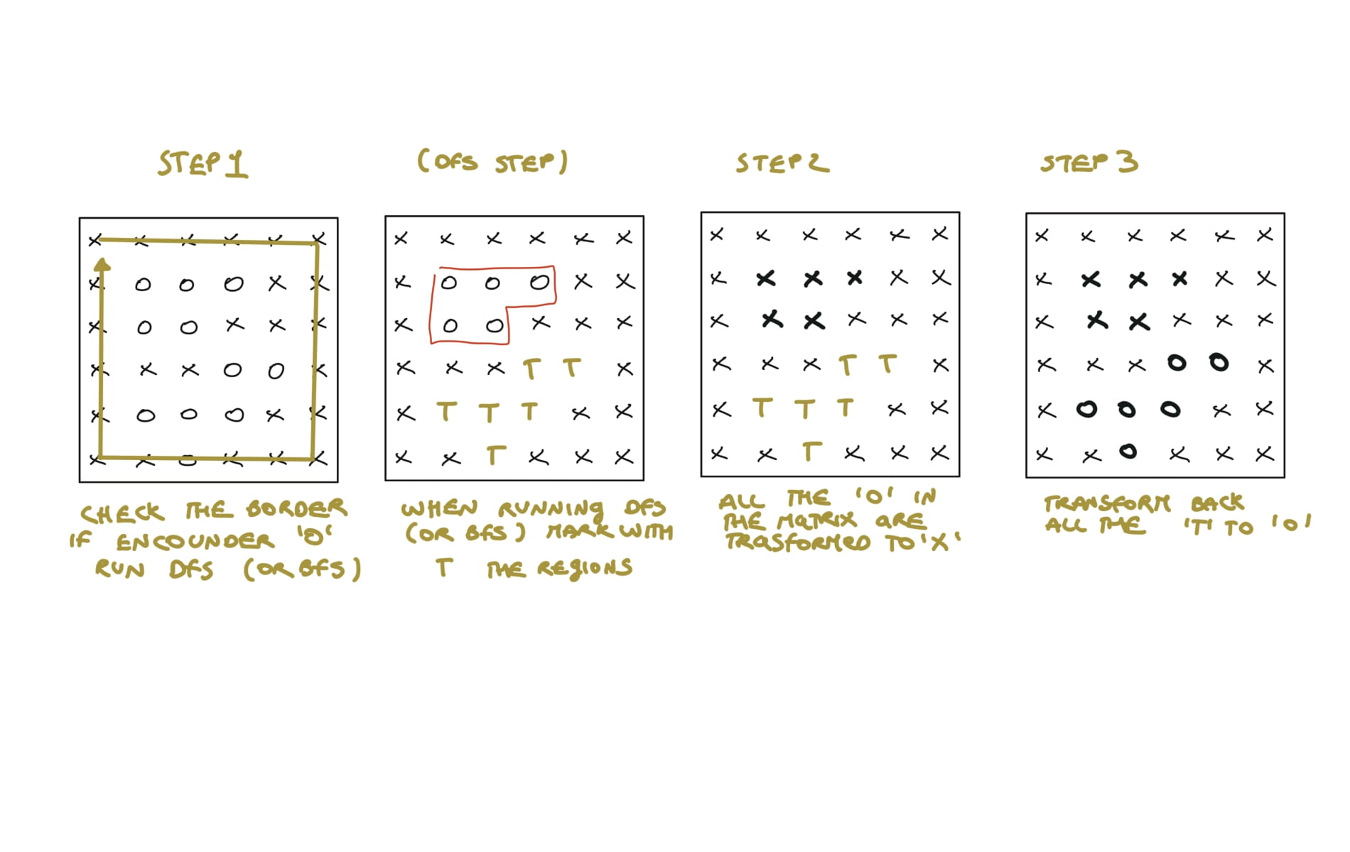
130. Surrounded Regions
[desc]
(link)
rows, cols= len(board), len(board[0])
def dfs(r,c):
    if (r<0 or r==rows or c<0 or c==cols or board[r][c]!="O"):
        return
    board[r][c]="T"
    dfs(r+1,c)
    dfs(r-1,c)
    dfs(r,c+1)
    dfs(r,c-1)
#(DFS)capture unsurrounded region(0->T)
for r in range(rows):
    for c in range(cols):
        if board[r][c]=="O" and (r==0 or r==rows-1 or c==0 or c==cols-1):
            dfs(r,c)
#capture surrounded region(0->x)
for r in range(1,rows-1):
    for c in range(1,cols-1):
        if board[r][c]=="O":
            board[r][c]="X"
#uncapture unsurrounded region(T->0)
for r in range(rows):
    for c in range(cols):
        if board[r][c]=="T":
            board[r][c]="O"
visualization
207. Course Schedule
[desc]
(link)
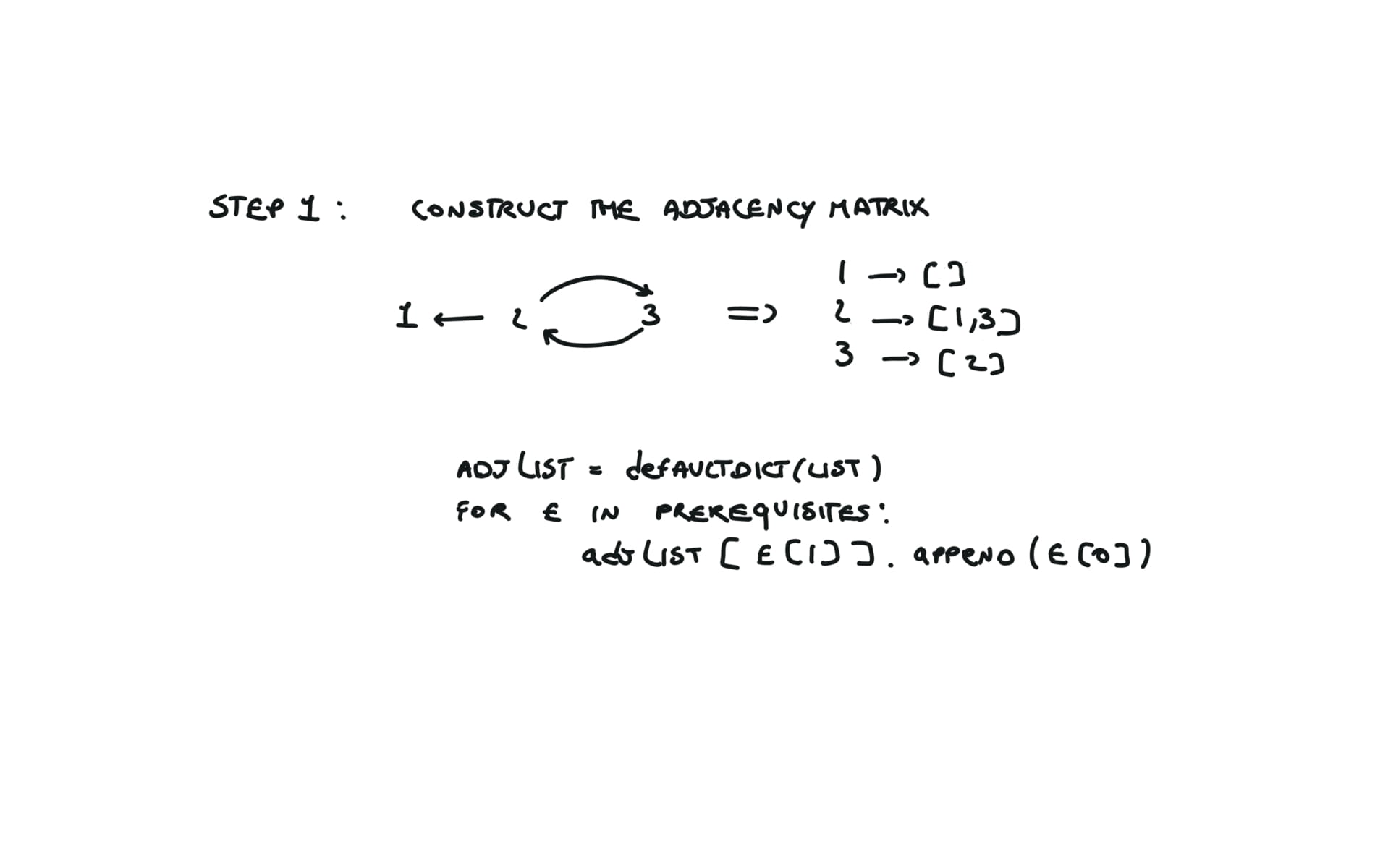
cycle detection or cycle detection with BFS topo sort
adjList = defaultdict(list)
for e in prerequisites:
    adjList[e[1]].append(e[0])

states = [0] * numCourses
def dfs(i):
    if states[i] == 2:
        return True
    states[i] = 1
    for v in adjList[i]:
        if states[v] == 1:
            return False
        a = dfs(v)
        if not a:
            return False
    states[i] = 2
    return True

for i in range(numCourses):
    if not dfs(i):
        return False
return True
visualization
using topological sort
adj_list = defaultdict(list)
for p in prerequisites:
    adj_list[p[1]].append(p[0])

in_degrees = [0] * numCourses
for p in prerequisites:
    in_degrees[p[0]] += 1

q = deque()
for i in range(numCourses):
    if in_degrees[i] == 0:
        q.append(i)
out = []
while q:
    v = q.popleft()
    out.append(v)
    for n in adj_list[v]:
        in_degrees[n] -= 1
        if in_degrees[n] == 0:
            q.append(n)

return len(out) == numCourses
210. Course Schedule II
[desc]
(link)
topological sort
adj_list = defaultdict(list)
for p in prerequisites:
    adj_list[p[1]].append(p[0])

in_degrees = [0] * numCourses
for p in prerequisites:
    in_degrees[p[0]] += 1

q = deque()
for i in range(numCourses):
    if in_degrees[i] == 0:
        q.append(i)
out = []
while q:
    v = q.popleft()
    out.append(v)
    for n in adj_list[v]:
        in_degrees[n] -= 1
        if in_degrees[n] == 0:
            q.append(n)
if len(out) == numCourses:
    return out
else:
    return []
Greedy
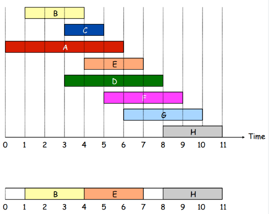
Problem: Suppose you have a resource shared by many people and it can’t be use in parallel. You have to maximize the number of task that can be done and return those tasks.
Greedy algorithms are about choosing at each step the best solution possible, and never looking back.
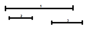
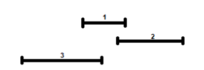
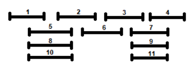
But what is the best solution in the case of the “interval scheduling” problem? I can choose the interval that starts first. But this one will lead to a non optimal solution.
I can choose the shortest interval first. But this one will lead to a non optimal solution.
I can choose the interval with the fewest conflicts. But this one will lead to a non optimal solution.
I can choose the interval that ends first. This one will lead to a non optimal solution. And this is the implementation in python: See the solution for interval-schedule, this algorithm is exactly that one but with a twist, here we don’t ask to return the right intervals but the number of intervals that are left out. Time complexity of the coin change problem (see 322. Coin Change) is
$$ O(N*K) $$ IF you have a canonical coin set (*) you can use a fully greedy approach.
In the case of problem 322 the testcase does not always have a canonical coin system, so we have to use a bruteforce approach (which is dynamic programming). The greedy choiche in this case is choosing at each step the largest coin that is less than the change.
The pseudo-code of the algorithm is the following: In python the code is: The algorithm requires a sort so: $$T(n) \in O(nlogn)$$interval-schedule
procedure IntervalSchedule (1,2,...,n)
	candidate <- {1,2,...,n}
	out <- {}
	while candidate
		k <- interval that ends first
		out <- out U {k}
		candidate <- candidate - {k}
		remove from candidate all the intervals incompatible with k
	return out
intervals.sort(key = lambda x: x[1])
out = [intervals[0]]
t = intervals[0][1]
for i in range(1,len(intervals)):
    if intervals[i][0] >= t:
		out.append(intervals[i])
        t = intervals[i][1]
return out
435. Non-overlapping Intervals
[desc]
(link)
intervals.sort(key = lambda x: x[1])
t = intervals[0][1]
out = 0
for i in range(1,len(intervals)):
    if intervals[i][0] >= t:
        t = intervals[i][1]
    else:
        out += 1
return out
coin change
def coinChange(change, coins):
	S = {}
	while change > 0:
		c = largest coins[i]: coins[i] <= r
		if no such c:
			return no solution
		change = change - c
		S = S + {c}
	return S
def coinChange(change, coins):
	out = []
	coins.sort()
	while r > 0 and coins:
		c = coins.pop()
		if c >= change:
			change = change - c
			out.append(c)
	if r == 0:
		return out
	else:
		return no solution
